By the end of this lecture, students should be able to:
Explain how integers, floating-point numbers, and ASCII text are represented in binary, and predict the size of a simple file from its content
Define information entropy and use it to bound the compressibility of a data source
Apply Huffman coding to an arbitrary string, and describe other common lossless techniques (run-length, dictionary-based) and where each performs well
Contrast lossless and lossy compression, and explain how frequency-domain (transform) representations enable lossy schemes such as JPEG
Apply delta and delta-of-delta encoding ideas to time-series data and estimate the achievable savings
Debate whether large language models are, in a meaningful sense, compression algorithms
NoteTopics Covered
Why size matters along the acquire → transmit → store pipeline
Binary representation of integers, floating-point numbers, and text; predicting file sizes
Information, entropy, and the limit it places on lossless compression
Lossless techniques: Huffman, run-length, and dictionary coding
Compressing time series with delta and delta-of-delta encoding
Lossy compression: transforms, quantization, JPEG, and feature extraction
Are large language models compressors? A debate
13.1.1 Before You Begin
This lecture compresses data you have already met, so it leans on two earlier chapters: Lecture 6, for the DFT and the two-story frame case study, and Lecture 8, for the office light-and-motion records and the storage formats compared at its end (Table 9.8 in that chapter). To follow along, save these files in a data/ folder next to your notebook:
The frame’s accelerometer records (SeismicResponse_noNoise.txt, collected by Matteo Pozzi) were shared with me for use in this course, not for public posting, so ask me or the TA for a copy if you want to run that example yourself.
Every code block in this chapter assumes that the setup below has run first, in the same Python session: it imports the libraries and defines the names the blocks share (see About the code in the Welcome chapter).
Chapter setup: imports and shared names
import collections, gzip, heapq, math, structimport numpy as npimport pandas as pdimport matplotlib.pyplot as pltfrom scipy.fft import dctn, idctndef entropy(symbols):"""Shannon entropy (bits per symbol) of the symbols' observed frequencies.""" n = np.array(list(collections.Counter(symbols).values()), dtype=float) p = n / n.sum()returnfloat(-(p * np.log2(p)).sum())def huffman_lengths(text):"""Code length of each symbol in a Huffman code built from the symbols' counts.""" counts = collections.Counter(text)iflen(counts) ==1:return {s: 1for s in counts} leaves =sorted(counts.items(), key=lambda kv: (kv[1], kv[0])) heap = [(n, i, [s]) for i, (s, n) inenumerate(leaves)] depth, order =dict.fromkeys(counts, 0), len(heap)whilelen(heap) >1: n1, _, a = heapq.heappop(heap) n2, _, b = heapq.heappop(heap)for s in a + b: depth[s] +=1 heapq.heappush(heap, (n1 + n2, order, a + b)) order +=1return depthdef canonical_codes(lengths):"""Prefix-free code words with the given lengths (shortest first).""" code, prev, words =0, None, {}for s, L insorted(lengths.items(), key=lambda kv: (kv[1], kv[0])):if prev isnotNone: code = (code +1) << (L - prev) words[s], prev =format(code, f"0{L}b"), Lreturn wordsdef lz77(s, window=255):"""Greedy LZ77: a list of (distance, length, next character) triples.""" i, out =0, []while i <len(s): best = (0, 0)for d inrange(1, min(i, window) +1): L =0while i + L <len(s) -1and s[i - d + L] == s[i + L]: L +=1if L > best[1]: best = (d, L) d, L = best out.append((d, L, s[i + L])) i += L +1return outroom = pd.read_csv("data/room_light_14d.csv") # 20,160 rows, one per minuteseis = np.loadtxt("data/SeismicResponse_noNoise.txt")FS =200# frame record: HzQ_ESP32 =3.3/4096# ESP32 12-bit converter step, V
13.2 Why Talk About Data Compression?
A hundred accelerometers sampling at 200 Hz produce 1.7 billion samples a day, about 3.5 GB even as two-byte integers, and every one of those bytes has to cross a radio link, land on a disk, and be read back by a query. Lecture 8 ended with a hint of how much the choice of representation matters: the same fourteen days of office data took 553 kB as plain text and less than a twentieth of that as a typed, delta-encoded Parquet file. This lecture explains where that factor comes from, and how far it can be pushed.
The data we have been studying moves through a pipeline: it is acquired at the sensor, transmitted over a network, and stored in files and databases. At each stage size costs something: bandwidth and battery for transmission, disk and money for storage, time for every query that has to read it back. Data compression means representing the same information in fewer bits, and its efficiency is measured by the compression ratio, \[
\text{compression ratio} = \frac{\text{original size}}{\text{compressed size}},
\tag{13.1}\] so a ratio of 4 means the compressed file is a quarter of the original. Compression comes in two kinds. A lossless scheme lets you reconstruct the original exactly, bit for bit; a lossy one discards information you have decided you do not need, and the reconstruction is only approximate. Both start from the same place: knowing how many bits the obvious representation spends, which is where we begin.
13.3 How Numbers and Text Become Bits
Before you can shrink a file you have to be able to predict its size, and that depends entirely on how each value is written in binary. Integers, floating-point numbers, and characters each have a standard encoding with a fixed or bounded cost per value, and those costs, added up, are the file size.
13.3.1 Integers
A 12-bit ADC code is an integer between 0 and 4095, and storing it costs whatever integer type you put it in, whether or not the bits are used. An unsigned integer of \(M\) bits holds the values \(0\) to \(2^M - 1\), each bit a power of two: the code 3173 is \(2^{11} + 2^{10} + 2^6 + 2^5 + 2^2 + 2^0\), or 110001100101 in binary. A signed integer uses two’s complement, which holds \(-2^{M-1}\) to \(2^{M-1} - 1\): the top bit carries the weight \(-2^{M-1}\) instead of \(+2^{M-1}\), so the same adder circuit works for negative and positive numbers alike. Computers offer these in four sizes (Table 13.1).
Table 13.1: The standard integer types.
Bits
Bytes
Unsigned range
Signed (two’s complement) range
8
1
0 to 255
-128 to 127
16
2
0 to 65,535
-32,768 to 32,767
32
4
0 to 4,294,967,295
-2,147,483,648 to 2,147,483,647
64
8
0 to \(2^{64} - 1 \approx 1.8 \times 10^{19}\)
\(\pm 9.2 \times 10^{18}\)
A 12-bit code fits in a 16-bit integer with four bits to spare; stored in Python’s default 64-bit integer, the same code costs four times as much. Choosing the smallest type that holds the range is the first and cheapest compression there is, and it is the one most often skipped, because the default types are large.
13.3.2 Floating-Point Numbers
Converting that code to volts turns an exact integer into a real number, and most real numbers cannot be written in any finite number of bits. Computers store them in the IEEE 754 floating-point format, scientific notation in base two: a sign bit \(s\), an exponent \(e\), and a fraction \(f\), representing \[
x = (-1)^s \times (1.f)_2 \times 2^{\,e - \text{bias}},
\tag{13.2}\] where \((1.f)_2\) is the binary number with a leading 1 and the fraction bits after the point (Goldberg 1991). A 32-bit single-precision float uses 1 sign bit, 8 exponent bits (bias 127), and 23 fraction bits; a 64-bit double uses 1, 11 (bias 1023), and 52. The 24 significant bits of a single (23 stored plus the implied leading 1) give about seven significant decimal digits; the 53 of a double give about sixteen.
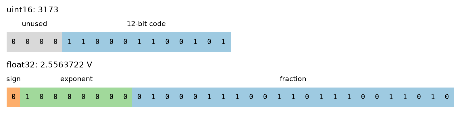
Going the other way, from a number \(x\) to its three fields, takes three steps. The sign bit \(s\) is 0 if \(x\) is positive and 1 if it is negative. The exponent is the power of two that brings \(|x|\) into the range from 1 to 2: \(e - \text{bias} = \lfloor \log_2 |x| \rfloor\), the largest integer not exceeding \(\log_2 |x|\). And the fraction is what is left after the leading 1 once \(|x|\) has been scaled into that range, \((1.f)_2 = |x| / 2^{\,e - \text{bias}}\): its part after the point is written in binary and rounded to the 23 bits available (52 in a double), and that rounding is the only error a float commits. Take the voltage of Figure 13.1 below, \(x = 3173 \times 3.3/4096 = 2.5563720703125\) V. It is positive, so \(s = 0\). Since \(2^1 \le x < 2^2\), \(\lfloor \log_2 x \rfloor = 1\) and the stored exponent is \(e = 1 + 127 = 128\), 10000000 in binary. Then \(x/2^1 = 1.27818603515625\), so the fraction is \(0.27818603515625\); scaled by \(2^{23}\) it is 2,333,593.6, which rounds to the integer 2,333,594, or 01000111001101110011010 in 23 bits. The value actually stored is \(2 \times (1 + 2{,}333{,}594/2^{23}) = 2.5563722\) V. This recipe covers ordinary (“normal”) numbers; zero, the tiniest numbers near it, the infinities, and NaN (“not a number”) use reserved exponent values, which the Wikipedia article on floating-point arithmetic describes along with the rest of the format.
Two consequences follow from Equation 13.2, and both bite in practice. First, the representable numbers are not evenly spaced: the gap between neighbours is proportional to the number’s magnitude, about \(10^{-7}\) of it for a single. Second, most decimal fractions are not representable at all, so they are rounded on the way in: the single nearest to 0.1 is 0.100000001490116…, and in double precision 0.1 + 0.2 evaluates to 0.30000000000000004. Neither is a bug; both are what a finite number of bits must do.
Figure 13.1 shows the ADXL335 example from Lecture 7 on its way to storage: the code 3173 from the ESP32’s 12-bit converter, and the voltage it stands for, \(3173 \times 3.3/4096 = 2.5564\) V, stored as a single.
Figure 13.1: One reading, two representations. Top: the ADC code 3173 in a 16-bit unsigned integer; the four leading bits are always zero for a 12-bit converter. Bottom: the same reading converted to volts (2.5564 V) and stored as a 32-bit float, split into sign (1 bit), exponent (8 bits), and fraction (23 bits).
The single in Figure 13.1 is not exactly 2.5564 V, but its error, about \(10^{-7}\) V, is four orders of magnitude below the converter’s own step of 0.8 mV, so for a voltage it is harmless. A single does real damage when the magnitude is large and the resolution matters, and the classic case in sensing is a timestamp. A Unix timestamp counts seconds since 1970; the first row of the fourteen-day record, 2025-11-10 05:00 UTC, is 1,762,750,800 s. Stored as a single, that number lies where neighbouring floats are 128 s apart, so four consecutive minutes collapse onto two values (Table 13.2), and a minute-resolution record becomes a two-minute one without any error message.
Table 13.2: The first four minutes of the fourteen-day record, with their timestamps stored as 32-bit floats. Neighbouring floats near \(1.76 \times 10^9\) are 128 s apart.
Minute
Unix time (s)
Stored as float32 (s)
Error (s)
0
1,762,750,800
1,762,750,848
+48
1
1,762,750,860
1,762,750,848
-12
2
1,762,750,920
1,762,750,976
+56
3
1,762,750,980
1,762,750,976
-4
Try it with your own numbers. Type any value below and the widget shows how a single stores it: the three fields, the value actually kept, and the gap to the next representable number.
fltOut = {const x =Number(fltIn), dv =newDataView(newArrayBuffer(4));if (!Number.isFinite(x)) returnhtml`<em>Type a finite number.</em>`; dv.setFloat32(0, x);const u = dv.getUint32(0), stored = dv.getFloat32(0), bits = u.toString(2).padStart(32,"0"); dv.setUint32(0, u +1);const gap =Math.abs(dv.getFloat32(0) - stored), exp =parseInt(bits.slice(1,9),2);returnhtml`<div style="font-family: monospace; font-size: 0.95em; line-height: 1.6"> <span style="background:#fdae6b">${bits[0]}</span><span style="background:#a1d99b">${bits.slice(1,9)}</span><span style="background:#9ecae1">${bits.slice(9)}</span><br> sign ${bits[0]} · exponent ${exp} − 127 = ${exp -127} · fraction 0.${bits.slice(9)}<br> stored value: ${stored.toPrecision(12)}<br> rounding error: ${(stored - x).toPrecision(4)}<br> gap to the next float: ${gap.toPrecision(4)}</div>`;}
The practical rules: store raw ADC codes as the small integers they are, and convert to physical units when you read them; if you must store physical values, a single is enough for most sensor readings and a double is needed for timestamps; and never store a timestamp as a single.
13.3.3 Text: ASCII and Unicode
A CSV file stores numbers as characters, so the code 3173 costs four bytes plus a comma instead of two bytes as an integer, and that is the price of a format anyone can read. Each character is mapped to bits by a character encoding, and two matter today. ASCII assigns each of 128 characters (English letters, digits, punctuation, and control characters such as the newline) a 7-bit code, stored in one byte: the digit 3 is 51, the comma 44, the newline 10. UTF-8 encodes every character in the Unicode standard, from Greek letters to emoji, in one to four bytes, and it was designed so that every ASCII character keeps its one-byte ASCII code: a file of plain ASCII text is a valid UTF-8 file. Characters outside ASCII cost more, two bytes for µ, ε, or °, and four for an emoji, so the 7-character string “1000 µε” occupies 9 bytes in UTF-8. Older systems also use UTF-16, two bytes for most characters and four for the rest, which doubles the size of English text and is efficient only for scripts, such as Chinese, that need three bytes per character in UTF-8.
13.3.4 Predicting a File’s Size
Knowing the per-value costs, you should be able to predict a file’s size before writing it, and that prediction is the baseline every compression ratio is measured against. A file’s size is the sum of its values’ encoded sizes plus delimiters and headers, and nothing more: the operating system adds no hidden overhead to the byte count it reports.
Try it on the fourteen-day record. Its first lines read:
The first data row is 2025-11-10T05:00:00Z,493,0: a 20-character timestamp, a comma, a three-digit code, a comma, a one-digit motion state, and a newline, 27 bytes. Rows whose code has four digits take 28. The header line, timestamp_utc,adc_code,pir_state, takes 33 bytes with its newline. Counting the rows of each length (Table 13.3) predicts the file’s size exactly. Stored instead as packed binary integers, with the timestamp as a 64-bit count of seconds, the code as a 16-bit integer, and the motion state as one byte, each row costs 11 bytes whatever the values, and a 32-bit timestamp would bring that to 7.
Table 13.3: Predicted sizes of the fourteen-day record (20,160 rows). The CSV prediction (a 33-byte header, 11,620 rows of 27 bytes, and 8,540 of 28) matches the file’s size on disk, 552,893 bytes, exactly.
Representation
Bytes per row
Total (kB)
Relative to CSV
CSV text
27.4
552.9
1.00
binary: int64 time, int16 code, uint8 state
11
221.8
0.40
binary: int32 time, int16 code, uint8 state
7
141.1
0.26
The packed forms are two and a half to four times smaller and say nothing that the CSV does not; all they give up is legibility. Everything else in this lecture starts from such a baseline and asks how much further the same information can shrink.
Type anything below to see what it costs in each encoding.
viewof txtIn = Inputs.textarea({label:"text",value:"Strain: 1000 µε at 23.5 °C",rows:2,width:420})
Before touching a computer, predict the number of bytes in one hour of the fourteen-day record written three ways: as CSV, as UTF-16 text, and as packed binary with a 32-bit timestamp. Then check your CSV and UTF-16 answers by pasting a few rows into the widget, and the binary one with len(struct.pack(...)). Where did your prediction go wrong, if it did?
13.4 Information and Entropy
Every compressor eventually meets a file it cannot shrink, so it is worth knowing, before trying, how small a file can get. In 1948 Claude Shannon answered that question by defining how much information a source produces, and showing that no lossless code can use fewer bits than that, on average (Shannon 1948).
13.4.1 Surprise and Information
A door sensor that reports “closed” ninety-nine times out of a hundred tells you almost nothing with each closed reading, and a great deal with each open one: the closed readings could be predicted, and the open ones could not. Information is a measure of that surprise. An outcome of probability \(p\) carries \[
I = -\log_2 p \quad \text{bits},
\tag{13.3}\] so a certain outcome (\(p = 1\)) carries none, a fair coin flip carries exactly one bit, and the door’s rare “open” (\(p = 0.01\)) carries 6.64 bits while each “closed” (\(p = 0.99\)) carries only 0.0145. The logarithm makes information add up for independent events, the way bits do: two coin flips carry two bits.
13.4.2 Entropy as a Compression Bound
Averaging that surprise over all the outcomes gives one number per source that says how compressible it is. The entropy of a source that emits symbol \(i\) with probability \(p_i\) is the expected information per symbol, \[
H = -\sum_i p_i \log_2 p_i \quad \text{bits per symbol},
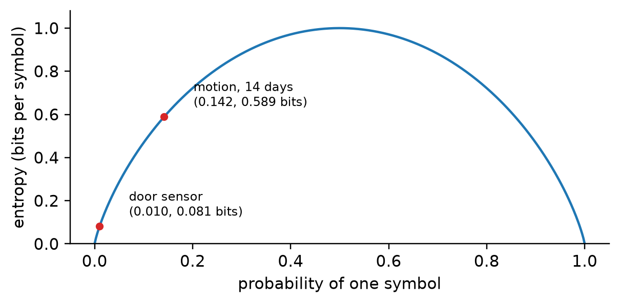
\tag{13.4}\] and Shannon’s source coding theorem says that no lossless code for symbols drawn independently from that source can average fewer than \(H\) bits per symbol, and that codes exist that come arbitrarily close (Shannon 1948; Sayood 2018). For the door sensor, \(H = -(0.01 \log_2 0.01 + 0.99 \log_2 0.99) = 0.081\) bits per reading: a hundred readings carry about eight bits of information, although writing each one as 0 or 1 in a CSV costs two bytes with its comma. The motion column of the fourteen-day record is a real two-symbol source of the same kind: 2,858 of its 20,160 readings are 1, a probability of 0.142, so its entropy is 0.589 bits per reading. For \(k\) equally likely symbols, \(H = \log_2 k\), the largest value any \(k\)-symbol source can reach; the more lopsided the probabilities, the lower the entropy and the more room there is to compress (Figure 13.2).
Figure 13.2: Entropy of a two-symbol source as the probability of one symbol varies. It peaks at 1 bit when both are equally likely. Marked: the door sensor (0.01, 0.081 bits) and the motion column of the fourteen-day record (0.142, 0.589 bits).
Two cautions keep the theorem honest. The bound is for symbols drawn independently: if successive symbols depend on each other, as they do in text and in every sensor record, a code that exploits the dependence can beat the single-symbol entropy, and the right comparison is the entropy of a better model of the source. And the probabilities are rarely known; in practice we estimate them from counts, which is what the entropy helper in the chapter setup does.
CautionConcept Check: The Universal Compressor
A vendor claims that their algorithm shrinks every file by at least one bit, losslessly. Should you buy it?
TipAnswer
No. Think of a compressor as a rule that turns each file it is given, its input (any sequence of bits), into an output file. For the rule to be lossless, no two inputs may share an output, or the decompressor could not tell which one to give back. Now count. There are \(2^n\) different inputs of exactly \(n\) bits, but only \(2^0 + 2^1 + \dots + 2^{n-1} = 2^n - 1\) bit strings shorter than \(n\) bits, counting the empty one. So the \(2^n\) inputs cannot all have distinct, shorter outputs: at least one of them must come out \(n\) bits long or longer. Every lossless compressor therefore makes some inputs longer; a good one arranges for those to be inputs nobody sends, such as random noise, and saves on the structured files people actually store.
A file of random bytes, each of the 256 possible values equally likely and independent of the others, is exactly such an input. Its entropy is \(\log_2 256 = 8\) bits per byte, which is just what storing the bytes as they are costs: the file has no redundancy left to remove, so no lossless code can average fewer than 8 bits per byte on it. That is what it means for the file to sit at the entropy bound. A compressor that tries anyway, such as gzip, finds no repeated phrases and no lopsided byte frequencies to exploit, and its output is the same random bytes plus its own header and bookkeeping: 100,000 random bytes come out of gzip as 100,053.
13.5 Lossless Compression
Legal records, raw sensor archives, and database files must come back bit for bit, so any compression applied to them has to be reversible. Lossless techniques approach the entropy bound by exploiting different kinds of redundancy: symbols that occur with unequal frequencies (Huffman coding), values that repeat in long runs (run-length encoding), and phrases that recur (dictionary coding).
13.5.1 Huffman Coding
A fixed-length code spends as many bits on a rare character as on a common one, which wastes bits whenever the frequencies are lopsided. Take the string “life liberty the pursuit of happiness”: 37 characters, 16 of them distinct. In ASCII it costs \(37 \times 8 = 296\) bits. Since 16 distinct symbols need only \(\lceil \log_2 16 \rceil = 4\) bits each, a fixed 4-bit code brings it to 148 bits. But the space occurs five times and the y once, and a code that gave the space a short word and the y a long one would save bits.
Variable-length codes have a catch: the decoder has to know where each code word ends. If the space were 0 and e were 01, the bits 01 could be e or a space followed by the start of something else. The fix is a prefix-free code, one in which no code word is the beginning of another; a stream of such code words can be cut into words unambiguously, left to right, with no separators. Among all prefix-free codes for given symbol counts, one uses the fewest total bits, and in 1952 David Huffman found how to build it (Huffman 1952):
Make one node per symbol, weighted by its count.
Remove the two nodes with the smallest weights and join them under a new node whose weight is their sum.
Repeat step 2 until one node remains: the root of a binary tree.
Read each symbol’s code word off the path from the root to its leaf, writing 0 for one branch and 1 for the other.
Frequent symbols are merged late and end up near the root, with short code words; rare ones are merged early and end up deep in the tree. The tree fixes each symbol’s code length; any prefix-free words with those lengths do equally well, and Table 13.4 uses the conventional choice of assigning them in order of length.
Table 13.4: A Huffman code for “life liberty the pursuit of happiness”. Bits = count × code length; the total is 142.
Symbol
Count
Code word
Bits
Symbol
Count
Code word
Bits
space
5
000
15
r
2
1001
8
e
4
001
12
u
2
1100
8
i
4
010
12
f
2
11100
10
p
3
1000
12
a
1
11010
5
s
3
1010
12
b
1
11011
5
t
3
1011
12
n
1
11101
5
h
2
0110
8
o
1
11110
5
l
2
0111
8
y
1
11111
5
The Huffman code needs 142 bits, 4% fewer than the fixed 4-bit code and 52% fewer than ASCII. How close is that to the best possible? Entropy answers that, and this is a good place to compute one by hand. Each symbol’s probability is its count divided by the 37 characters, and symbols with the same count contribute equally to Equation 13.4, so group them: one symbol (the space) occurs 5 times, two (e, i) 4 times, three (p, s, t) 3 times, five (f, h, l, r, u) twice, and five (a, b, n, o, y) once. Then \[
\begin{aligned}
H &= -\Big[\,1 \cdot \tfrac{5}{37}\log_2\tfrac{5}{37} + 2 \cdot \tfrac{4}{37}\log_2\tfrac{4}{37} + 3 \cdot \tfrac{3}{37}\log_2\tfrac{3}{37} + 5 \cdot \tfrac{2}{37}\log_2\tfrac{2}{37} + 5 \cdot \tfrac{1}{37}\log_2\tfrac{1}{37}\,\Big] \\
&= 0.3902 + 0.6939 + 0.8816 + 1.1377 + 0.7040 = 3.807 \text{ bits per symbol}.
\end{aligned}
\] That is the average information per character. The entropy bound for the whole string adds up the information of all 37 characters: each occurrence of symbol \(i\) carries \(-\log_2 p_i\) bits (Equation 13.3), so the total is \(\sum_i n_i(-\log_2 p_i) = N H = 37 \times 3.807 = 140.9\) bits, where \(n_i\) is the count of symbol \(i\) and \(N\) the length of the string. No prefix-free code for these frequencies can use fewer. The Huffman code averages \(142/37 = 3.838\) bits per symbol, 1.1 bits above the bound over the whole string. In general, for a source with at least two symbols, a Huffman code’s average length \(\bar L\) satisfies \[
H \le \bar L < H + 1,
\tag{13.5}\] and it equals \(H\) exactly when every probability is a power of \(1/2\)(Sayood 2018). Three properties decide where Huffman coding is worth using. It is optimal among codes that assign each symbol its own whole number of bits. The decoder needs the code table, which has to be stored or sent along with the data, so short messages gain little. And it can never spend less than one bit per symbol, which wastes most of the bits on a lopsided source like the door sensor, whose entropy is 0.081 bits per reading.
Build a code for any text you like below, and watch the encoded length chase the entropy bound.
viewof hufIn = Inputs.textarea({label:"text",value:"life liberty the pursuit of happiness",rows:2,width:420})
hufOut = {const sym = [...hufIn], n = sym.length;if (n ===0) returnhtml`<em>Type some text.</em>`;const counts =newMap();for (const c of sym) counts.set(c, (counts.get(c) ||0) +1);const leaves = [...counts.entries()].sort((a, b) => a[1] - b[1] || (a[0] < b[0] ?-1: a[0] > b[0] ?1:0));const depth =newMap(leaves.map(([c]) => [c,0]));let nodes = leaves.map(([c, w], i) => ({w,o: i,s: [c]})), order = nodes.length;if (nodes.length===1) depth.set(leaves[0][0],1);while (nodes.length>1) { nodes.sort((a, b) => a.w- b.w|| a.o- b.o);const [a, b] = nodes.splice(0,2);for (const c of [...a.s,...b.s]) depth.set(c, depth.get(c) +1); nodes.push({w: a.w+ b.w,o: order++,s: [...a.s,...b.s]}); }const byLen = [...depth.entries()].sort((a, b) => a[1] - b[1] || (a[0] < b[0] ?-1: a[0] > b[0] ?1:0));let code =0, prev =null;const words =newMap();for (const [c, L] of byLen) { if (prev !==null) code = (code +1) *2** (L - prev); words.set(c, code.toString(2).padStart(L,"0")); prev = L; }const k = counts.size, bitsH = [...counts].reduce((t, [c, m]) => t + m * depth.get(c),0);const H =-[...counts.values()].reduce((t, m) => t + (m / n) *Math.log2(m / n),0);const show = c => c ===" "?"space": c ==="\n"?"newline": c;const rows = [...counts.entries()].sort((a, b) => b[1] - a[1] || depth.get(a[0]) - depth.get(b[0]) || (a[0] < b[0] ?-1:1));returnhtml`<div style="font-size: 0.95em"> <p>${n} symbols, ${k} distinct · ASCII: <b>${8* n}</b> bits · fixed-length: <b>${Math.max(1,Math.ceil(Math.log2(k))) * n}</b> bits · Huffman: <b>${bitsH}</b> bits · entropy bound: <b>${(n * H).toFixed(1)}</b> bits (${H.toFixed(3)} bits/symbol)</p> <div style="max-height: 260px; overflow-y: auto"><table style="width: auto"><tr><th>symbol</th><th>count</th><th>code word</th><th>bits</th></tr>${rows.map(([c, m]) =>html`<tr><td>${show(c)}</td><td>${m}</td><td style="font-family: monospace">${words.get(c)}</td><td>${m * depth.get(c)}</td></tr>`)} </table></div></div>`;}
TipActive Learning: Code a Pump’s Status Log
A water utility’s SCADA system logs a booster pump’s status every hour as one letter: R (running), S (stopped), M (maintenance), or F (fault). One day’s log reads RRRRSRRRMRRSSRRRSSMF: twelve Rs, five Ss, two Ms, and one F. By hand, build the Huffman tree, write down the code words, and count the bits; compare with a fixed 2-bit code and with the entropy bound. Then check your answer in the widget above.
TipAnswer
Merge F (1) and M (2) into a node of 3; merge it with S (5) into 8; merge that with R (12) into 20. The code lengths are R 1, S 2, M 3, F 3, for example R = 0, S = 10, M = 110, F = 111, and the log costs \(12 + 10 + 6 + 3 = 31\) bits, against 40 with a fixed 2-bit code. The entropy is 1.490 bits per symbol, a floor of 29.8 bits.
13.5.2 Run-Length Encoding
The motion column of the fourteen-day record sits at 0 for hours at a time, and Huffman coding cannot spend less than a bit on each of those zeros. Run-length encoding (RLE) replaces each run of identical values by the value and the run’s length, so BBWWWWBBBBBBWBBBBBBBBWW (23 characters) becomes 2B4W6B1W8B2W (12). It is tiny for long runs and counterproductive without them: abcdefgh becomes 1a1b1c1d1e1f1g1h, twice as long.
The motion column shows both cases within a few hours. It opens with 497 zeros, from midnight until 08:16 on Monday, before anyone walks in: as a run, that is a single (count, value) pair. The next sixty minutes, with the office occupied, read
and break into 37 runs, so run-length encoding that hour replaces 60 readings by 37 pairs, a loss rather than a saving. RLE pays where the data rest.
RLE is also the clearest example of the caution in Section 13.4.2. Treated as independent symbols, the motion column’s 20,160 readings have an entropy of 0.589 bits each, a floor of 11,871 bits. But the readings are not independent: a 0 is usually followed by another 0. The column consists of 2,577 runs, and if the runs’ lengths are themselves entropy-coded, the floor drops to 5,794 bits, half the “bound”. RLE did not beat Shannon; it used a better model of the source (runs, rather than independent readings), and a better model has a lower entropy. RLE earns its keep on binary images such as scanned drawings, on sensor streams that rest at one value, and, as JPEG will show, on lists of coefficients that are mostly zero.
13.5.3 Dictionary Coding
Text, logs, and CSV files repeat whole words and phrases, not just characters, and a code that looks at one symbol at a time cannot see that. Dictionary coders replace a repeated phrase by a reference to an earlier occurrence. The LZ77 scheme of Ziv and Lempel (Ziv and Lempel 1977) slides along the text and, at each position, looks back for the longest match with what comes next; it emits a triple (distance back, length of the match, next character) and jumps past the match. Table 13.5 traces it on a short pump log,
pump on; pump off; pump on; pump off;
The first occurrence of each phrase is spelled out character by character; the second pump on; pump off; is copied in two triples.
Table 13.5: LZ77 on “pump on; pump off; pump on; pump off;” (37 characters, 12 triples; ␣ marks a space). A triple with length 0 is a literal character.
Step
Triple (distance, length, next)
Text produced
1
(0, 0, p)
p
2
(0, 0, u)
u
3
(0, 0, m)
m
4
(3, 1, ␣)
p␣
5
(0, 0, o)
o
6
(0, 0, n)
n
7
(0, 0, ;)
;
8
(4, 1, p)
␣p
9
(9, 5, f)
ump␣of
10
(1, 1, ;)
f;
11
(10, 7, n)
␣pump␣on
12
(19, 10, ;)
;␣pump␣off;
On 37 characters the saving is modest, because each triple costs more than a character. On real files it is large: gzip, which combines LZ77 with Huffman coding of the triples, shrinks the fourteen-day CSV from 553 kB to 76 kB, a ratio of 7.3. Treating the same file’s bytes as independent symbols, their entropy is 3.65 bits per byte, so even a perfect Huffman code could reach a ratio of only \(8/3.65 = 2.2\): LZ77 wins by modelling repeated phrases, here the timestamps’ long shared prefixes, visible in the first lines of the file in Section 13.3.4. A variant by Welch, LZW (Welch 1984), builds an explicit dictionary of phrases as it goes, and the family is inside zip, gzip, PNG, and GIF. Dictionary coders shine on text, logs, and markup; they do little for noisy numeric data, in which phrases rarely repeat exactly.
13.6 Compressing Time Series: Delta and Delta-of-Delta
Lecture 8 found that a delta-encoded Parquet file stored the fourteen-day record in 19 kB, under a twentieth of the CSV and a quarter of the gzip file. The reason is that consecutive readings of a physical quantity, and consecutive timestamps, differ by small and predictable amounts, so storing the differences turns large values with high entropy into small values with low entropy, which a variable-length code then packs into a few bits each.
Delta encoding stores the first value and then the differences \[
\Delta x_i = x_i - x_{i-1},
\tag{13.6}\] from which the decoder rebuilds every value by a running sum, so nothing is lost. Delta-of-delta encoding differences once more, \[
\Delta^2 x_i = \Delta x_i - \Delta x_{i-1},
\tag{13.7}\] which is zero wherever the series moves in a straight line. Timestamps are the ideal case: a logger that writes a row every 60 s produces deltas of 60 and delta-of-deltas of 0, which carry no information at all. Facebook’s Gorilla time-series database builds its compression on exactly these ideas, delta-of-delta for timestamps and a related trick for values, and reports that about 96% of its timestamps compress to a single bit and its points from 16 bytes to 1.37 bytes on average (Pelkonen et al. 2015).
Table 13.6 shows both transforms on eight minutes of the record, around the moment the lights came on on Monday morning.
Table 13.6: Eight minutes of the fourteen-day record (Monday 08:14 to 08:21 local time), with the deltas and delta-of-deltas of the codes and of the timestamps. The lights came on at 13:18 UTC.
Time (UTC)
Code
\(\Delta\) code
\(\Delta^2\) code
\(\Delta\) time (s)
\(\Delta^2\) time (s)
13:14
2598
13:15
2596
-2
60
13:16
2573
-23
-21
60
0
13:17
2587
+14
+37
60
0
13:18
3591
+1004
+990
60
0
13:19
3589
-2
-1006
60
0
13:20
3594
+5
+7
60
0
13:21
3595
+1
-4
60
0
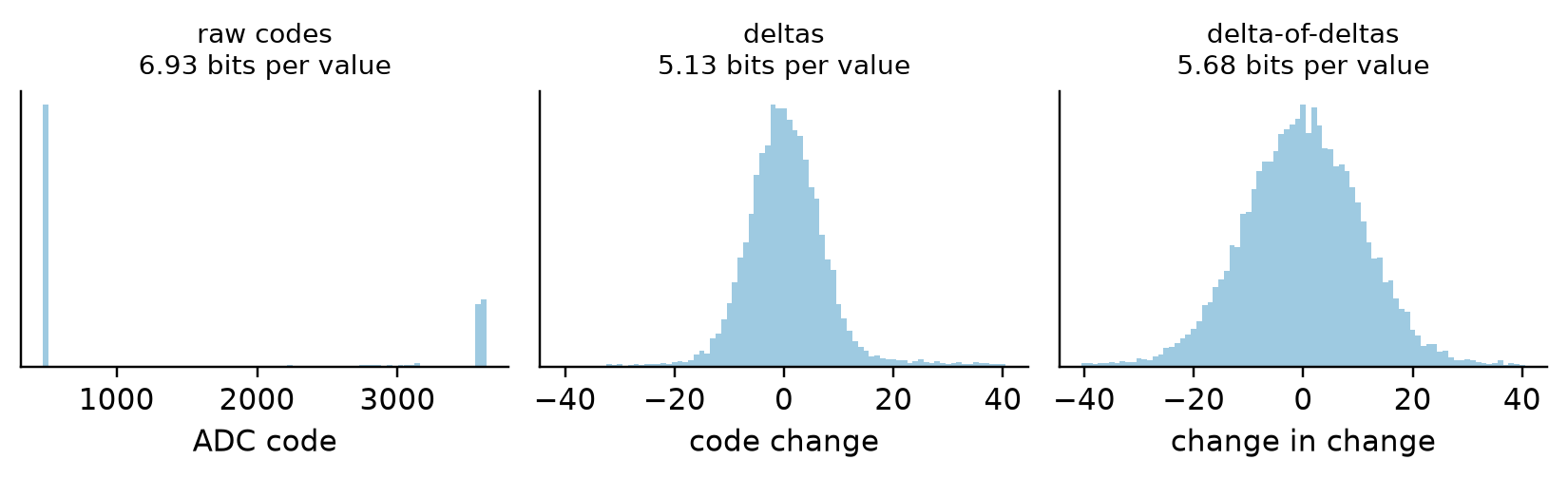
The timestamps’ deltas are always 60 and their delta-of-deltas always 0. The codes’ deltas are a few counts, except for the jump of 1004 when the lights switched on, and their delta-of-deltas are no smaller: every second difference mixes two of the noisy steps, and the one jump appears twice, once going up and once coming back. Which transform helps depends on the series. In the fourteen-day record, every timestamp delta is 60 s, so the timestamps’ delta-of-deltas are all zero and have zero entropy. The ADC codes, raw, have an entropy of 6.93 bits per value; their deltas, 5.13 bits; and their delta-of-deltas, 5.68 bits, more than the deltas (Figure 13.3). Differencing removes the slowly varying part of a signal but adds noise: if successive noise samples are independent, each difference subtracts two of them, doubling the noise variance, and a second difference triples it again. Delta-of-delta pays off for smooth series such as timestamps and counters; for noisy measurements, a single delta is usually the sweet spot.
Figure 13.3: Distributions of the fourteen-day record’s ADC codes, their deltas, and their delta-of-deltas, with the entropy of each. The deltas cluster near zero, except for the jumps when the lights switch; the second difference spreads the noise wider again. The horizontal axes of the last two panels are clipped at ±40 codes.
Put together, the column-by-column entropies estimate what a good delta-based encoder can achieve on this record. Timestamps cost essentially nothing after the first; the codes, delta-encoded, about 5.13 bits per row; and the motion state, even treated as independent readings, 0.59 bits per row. That is about 5.7 bits, or 0.72 bytes, per row, against 27.4 bytes as CSV, a ratio of about 38. Lecture 8’s delta-encoded Parquet file, at 0.96 bytes per row, came within a factor of 1.3 of this estimate using only general-purpose encodings.
Explore the codes of one day below: switch between the raw series, its deltas, and its delta-of-deltas, and watch the histogram, and the entropy, change.
dOut = {const x = dayCodes, d1 = x.slice(1).map((v, i) => v - x[i]), d2 = d1.slice(1).map((v, i) => v - d1[i]);const v = dSel ==="raw codes"? x : dSel ==="deltas"? d1 : d2, n = v.length, cnt =newMap();for (const a of v) cnt.set(a, (cnt.get(a) ||0) +1);const H =-[...cnt.values()].reduce((t, m) => t + (m / n) *Math.log2(m / n),0);const pts = v.map((y, i) => ({h: (i + (x.length- n)) /60, y}));const series = Plot.plot({width:Math.min(720, width),height:200,marginLeft:50,x: {label:"hours since Monday 00:00 EST",domain: [0,24],ticks: d3.range(0,25,3)},y: {label: dSel},marks: [Plot.line(pts, {x:"h",y:"y",stroke:"#1f77b4",strokeWidth:0.8}), Plot.ruleY([0], {stroke:"0.7"})]});const clip = dSel ==="raw codes"? v : v.filter(a =>Math.abs(a) <=40);const hist = Plot.plot({width:Math.min(720, width),height:170,marginLeft:50,x: {label: dSel ==="raw codes"?"ADC code":"value (clipped at ±40)"},y: {label:"count"},marks: [Plot.rectY(clip, Plot.binX({y:"count"}, {x: d => d,thresholds: dSel ==="raw codes"?60:81,fill:"#9ecae1"})), Plot.ruleY([0])]});returnhtml`<div><p style="margin: 0.3em 0"><b>${H.toFixed(2)} bits per value</b> over ${n} values</p>${series}${hist}</div>`;}
CautionConcept Check: When Does Differencing Help?
A data logger records a building’s cumulative electricity meter (kWh, a counter that only increases) and a room’s air temperature, each once a minute. For which would you expect delta-of-delta encoding to beat plain delta encoding, and why?
TipAnswer
The meter. Its deltas are the minute-by-minute consumption, which changes slowly, so the delta-of-deltas cluster tightly around zero. The temperature is a slowly varying signal plus sensor noise; its deltas are already small, mostly noise, and a second difference only adds noise, as it did for the ADC codes in Figure 13.3.
ImportantExercise: A Year of a Hundred Kits
A campus deploys a hundred Lecture 8 kits, each logging one row a minute like the fourteen-day record. Estimate the storage for one year of data from all of them as CSV, as packed binary rows (11 bytes), and with delta-based encoding at the entropy estimate of this section. Which column do the savings come from?
TipSolution
A year has \(365 \times 1440 = 525{,}600\) minutes, so the hundred kits write \(52{,}560{,}000\) rows. As CSV at 27.4 bytes per row, that is 1.44 GB; as packed rows, 0.58 GB; delta-encoded at about 0.72 bytes per row, 38 MB. The packed format saves by dropping characters; the delta encoding saves mostly on the timestamps, which become free, and on the codes, which drop from 16 bits to about 5.
13.7 Lossy Compression
For a vibration record, a photograph, or a sound, you care about features of the data, not every bit, and keeping every bit costs far more than the features need. Lossy compression discards information the application can do without, trading a reconstruction error for compression ratios that no lossless scheme can reach; the engineering question is always which information is expendable, and how much error the application tolerates.
13.7.1 Change of Basis to Uncover Structure
In Lecture 6 the response of the two-story frame looked like 5000 unrelated samples in time, and like a handful of peaks in frequency. The DFT is a change of basis: it rewrites the same 5000 numbers as the amplitudes and phases of sinusoids, and it loses nothing, since the inverse DFT gives the samples back exactly. What it changes is where the signal’s energy sits. In time, the energy of a vibration record is spread across all the samples; in frequency, most of it is concentrated in the few coefficients near the structure’s modes, and most of the remaining coefficients are small. A lossy coder exploits exactly that: it keeps what is large and drops what is small, and the basis is chosen to make as much as possible small.
13.7.2 From Representation to Compression
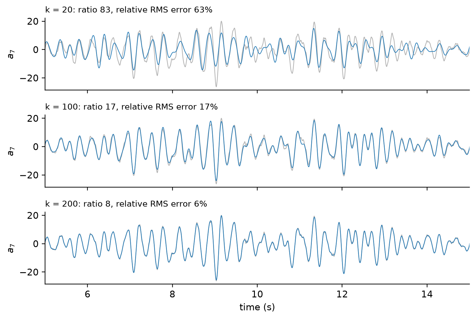
If a few coefficients carry most of the energy, the rest are candidates for deletion. Keep the \(k\) largest DFT coefficients of a real signal of \(N\) samples, each with its frequency index, real part, and imaginary part (amplitude and phase: without the phase, the reconstruction would be a different signal), set the others to zero, and invert. The stored record shrinks from \(N\) numbers to \(3k\), a compression ratio of \(N/3k\), and the error grows as \(k\) shrinks. Figure 13.4 shows the trade on channel \(a_7\) of the frame record, with the error measured as the RMS difference between the reconstruction and the original, relative to the RMS of the original.
Show the code
x = seis[:, 6]; N =len(x); t = np.arange(N) / FSX = np.fft.rfft(x)largest = np.argsort(np.abs(X))[::-1]def topk(k): Y = np.zeros_like(X); Y[largest[:k]] = X[largest[:k]] y = np.fft.irfft(Y, N)return y, np.sqrt(np.mean((x - y)**2) / np.mean(x**2))fig, axs = plt.subplots(3, 1, figsize=(7.4, 5.0), sharex=True, sharey=True)for ax, k inzip(axs, (20, 100, 200)): y, err = topk(k) ax.plot(t, x, color="0.7", lw=0.8); ax.plot(t, y, color="#1f77b4", lw=0.7) ax.set_title(f"k = {k}: ratio {N / (3* k):.0f}, relative RMS error {100* err:.0f}%", fontsize=9, loc="left") ax.set_ylabel("$a_7$")axs[-1].set_xlabel("time (s)"); axs[-1].set_xlim(5, 15)fig.tight_layout(); plt.show()
Figure 13.4: Channel \(a_7\) of the two-story frame record (gray) and its reconstruction (blue) from the \(k\) largest of its 2501 DFT coefficients, for three values of \(k\). Each panel gives the compression ratio \(N/3k\) and the relative RMS error.
Table 13.7: Compression ratio and error for truncated DFTs of channel \(a_7\).
\(k\)
Compression ratio \(N/3k\)
Relative RMS error
10
166.7
76.5%
50
33.3
36.6%
100
16.7
17.1%
150
11.1
8.5%
200
8.3
5.7%
300
5.6
3.7%
The numbers are sobering. Ten coefficients, a ratio of 167, leave an error of more than three quarters of the signal’s RMS; a 6% error needs about 200, a ratio of only 8. The frame record is a transient: the shaking starts, grows, and decays, and a signal that changes in time needs many sinusoids, each lasting the whole record, to cancel each other where it is quiet. That is a property of the basis, not of the idea, and it is why practical coders transform short blocks rather than whole records, and why the transforms behind JPEG and MP3 work on blocks of a few samples or pixels at a time.
13.7.3 JPEG Image Compression
Photographs from bridge inspections and drone surveys are stored as JPEG files, typically at a tenth of their raw size or smaller with no difference visible to the eye. JPEG, standardized in 1992, assembles everything in this lecture into one pipeline (Wallace 1992):
Color conversion. The red, green, and blue channels are converted to one brightness (luminance) and two color (chrominance) channels. The eye is more sensitive to brightness than to color, so the color channels are usually stored at reduced resolution.
Blocks. Each channel is cut into 8×8 blocks of pixels.
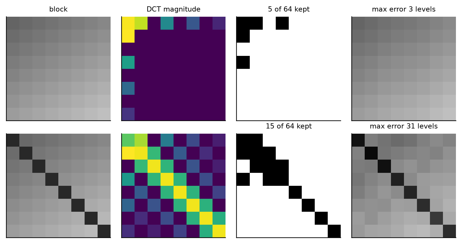
Transform. Each block goes through the two-dimensional discrete cosine transform (DCT), a relative of the DFT that uses only cosines. Its 64 coefficients run from the block’s average brightness (top left) to the finest checkerboard detail (bottom right), and, as with the frame record’s spectrum, a typical block’s energy sits in a few low-frequency coefficients.
Quantization. Each coefficient \(C\) is divided by an entry of a quantization table and rounded, \(\hat C = \operatorname{round}(C/Q)\). The table’s entries grow toward high frequencies, which the eye barely notices, so most high-frequency coefficients round to zero. This is the only lossy step, and JPEG’s quality setting scales the table.
Lossless coding. The quantized coefficients are read in a zigzag from low to high frequency, which collects the zeros into long runs, and are coded with run-length and Huffman coding.
Figure 13.5 runs steps 3 and 4 on two synthetic 8×8 blocks with the standard luminance quantization table: a smooth gradient, like a patch of sky or a concrete surface, and the same gradient crossed by a dark diagonal, like a crack.
Figure 13.5: JPEG’s transform and quantization on two 8×8 blocks: a smooth gradient (top) and a gradient crossed by a dark diagonal (bottom). From left: the block, the magnitudes of its 64 DCT coefficients (log scale), the coefficients left nonzero after quantization with the standard luminance table, and the block rebuilt from them.
The smooth block survives as 5 of its 64 coefficients and comes back within 3 gray levels of the original; the crack, a sharp feature, keeps three times as many coefficients and still comes back blurred, with errors of up to 31 levels around the line, which is the source of the “ringing” around sharp edges in heavily compressed JPEGs. For an inspection photograph, that is a warning worth heeding: the detail JPEG discards first, fine high-contrast lines, is exactly what a crack looks like.
13.7.4 Feature Extraction: A Different Kind of Compression
A structural health monitoring system rarely needs the raw waveform from a quiet night, only evidence that nothing happened. Feature extraction keeps only quantities computed from the data, such as the mean, standard deviation, and peak of each one-second window, and discards the samples. For one channel of the frame record, 25 one-second windows with three features each replace 5000 samples by 75 numbers, a ratio of 67; many monitoring systems go further and transmit the raw samples only when a feature crosses a threshold, so a quiet day costs almost nothing.
This is the most extreme lossy compression of all, because the original can never be reconstructed from the features, and it works only if you knew in advance which features matter. A record kept only as hourly averages cannot later be searched for a ten-second event. Table 13.8 summarizes the three families of this lecture.
Table 13.8: Three families of compression. The ratios are those of this lecture’s examples.
Approach
Typical ratio
Reconstruction
Typical use
Lossless (Huffman, RLE, LZ77, delta)
2–40 on sensor data
exact
archives, raw records, databases
Transform with quantization (DCT, truncated DFT)
10 or more
approximate
images, audio, vibration
Feature extraction
100 or more
none: features only
monitoring, event detection
13.8 Is a Language Model a Compressor?
A model that predicts the next word well needs very few bits to encode the word that actually comes next, which suggests that prediction and compression are the same problem in different clothes. The idea has a precise form. Arithmetic coding, a successor to Huffman coding, encodes a whole message as one number and spends, for each symbol, almost exactly \(-\log_2 p\) bits, where \(p\) is the probability a model assigned to that symbol before seeing it (Equation 13.3), so it is not limited to whole bits per symbol (Sayood 2018). A model that gives the next word a probability of 1/2 costs one bit to encode it; one that gives it 1/1024, ten bits. Any model that predicts well, paired with an arithmetic coder, is therefore a lossless compressor, and the better it predicts, the shorter the code.
Delétang and colleagues took this literally (Delétang et al. 2024). Paired with an arithmetic coder, the language model Chinchilla 70B compressed a gigabyte of Wikipedia text (the enwik9 benchmark) to 8.3% of its size, against 32.3% for gzip. But the decoder needs the model, and once the model’s own size is counted as part of the compressed file, the same model “compresses” that gigabyte to 14,008% of its size. Ted Chiang argued the opposite case a year earlier, in an essay that borrows this lecture’s vocabulary: a language model, he wrote, is “a blurry JPEG of the web” (Chiang 2023), a lossy compression of its training text that keeps the statistical gist and, where it has lost the details, interpolates plausible ones.
TipActive Learning: The Debate
Before class, read Chiang’s essay (about fifteen minutes) and the abstract and Section 1 of Delétang et al. In class, half the room argues that a large language model is, in a meaningful sense, a compression algorithm, and the other half that it is not. Each side must use at least three ideas from this lecture as evidence: entropy and the source coding theorem, lossless versus lossy, the cost of the code table (or the model), the difference between compressing a file and summarizing a corpus, and JPEG’s quantization step. Questions worth fighting over: Is a model that can regenerate its training text exactly a lossless compressor, and one that cannot a lossy one? Does a compressor need a decompressor that gives back the original, or is “something like it” enough? And what, exactly, is the original?
13.9 Putting It All Together
Every representation choice in this lecture, from the integer type of an ADC code to the \(k\) of a truncated DFT, sets how many bits a reading costs on its way from the sensor to the database. Entropy says how far lossless methods can push that cost for a given model of the data; Huffman, run-length, dictionary, and delta coding are different models, each matched to a different kind of redundancy; and lossy methods go further by deciding which information the application can do without. The MODELS third starts from data shaped by exactly these choices. And the MODELS third of the course leans on this lecture’s last idea: a model that captures the structure of the data is, in a precise sense, a good compressor of it.
13.10 Exercises
A bridge’s monitoring system logs eight accelerometer channels at 200 Hz as 12-bit ADC codes. Predict the size of one day of data, ignoring timestamps:
as CSV text, assuming each code is written with four digits and followed by one delimiter;
as packed 16-bit integers;
as the voltages, stored as 64-bit floats.
TipSolution
One day is \(200 \times 86{,}400 = 17{,}280{,}000\) samples per channel, or \(138{,}240{,}000\) values for eight channels.
At 5 bytes per value, 691.2 MB.
At 2 bytes per value, 276.5 MB.
At 8 bytes per value, 1.11 GB, four times the packed integers, for no gain in information: the voltages are a fixed multiple of the codes.
An occupancy sensor classifies a room as empty, low, medium, or high every five minutes, with long-run probabilities 1/2, 1/4, 1/8, and 1/8.
What is the entropy of one reading, and how many bits would a fixed-length code spend?
What is the smallest number of bytes in which a year of readings could be stored losslessly, if successive readings were independent?
Why might the real data compress further than (b) says?
TipSolution
\(H = \tfrac12 \cdot 1 + \tfrac14 \cdot 2 + \tfrac18 \cdot 3 + \tfrac18 \cdot 3 = 1.75\) bits per reading; a fixed-length code for four symbols spends 2. Because every probability is a power of 1/2, a Huffman code (0, 10, 110, 111) reaches 1.75 exactly.
A year has \(365 \times 288 = 105{,}120\) readings, so \(105{,}120 \times 1.75 = 183{,}960\) bits, or 22,995 bytes.
Successive readings are not independent: an empty room at 3 a.m. is very likely still empty five minutes later. A model that conditions on the previous reading, or run-length encoding, can go below the independent-symbol bound.
A valve on a water main reports its state each minute as O (open), C (closed), T (travelling), or F (fault). In one twenty-minute stretch it reports O ten times, C five times, T three times, and F twice.
Build a Huffman code and find the encoded length of the twenty readings.
Compare it with a fixed-length code and with the entropy bound.
TipSolution
Merge F (2) and T (3) into 5; merge that with C (5) into 10; merge that with O (10) into 20. The code lengths are O 1, C 2, T 3, F 3 (for example O = 0, C = 10, T = 110, F = 111), and the readings cost \(10 + 10 + 9 + 6 = 35\) bits.
A fixed 2-bit code costs 40 bits. The entropy is 1.743 bits per reading, a floor of 34.9 bits, so the Huffman code is within a fraction of a bit of the bound.
For each data stream, say which lossless technique (Huffman, run-length, dictionary, or delta coding) you would try first, and why:
a motion sensor sampled once a second in an office that is empty at night;
a text log in which a SCADA system writes lines such as 2026-10-03 14:02:11 PUMP-07 STATUS OK;
a water level sensor in a reservoir, logged every minute as a 16-bit integer.
TipSolution
Run-length encoding: the stream rests at “no motion” for hours, so runs are long.
Dictionary coding (gzip): device names, status words, and the date prefix repeat line after line.
Delta coding: the level changes slowly, so successive differences are small integers near zero, which a variable-length code then packs into a few bits each.
Using Table 13.7, choose the number of DFT coefficients \(k\) for channel \(a_7\) that keeps the relative RMS error at or below 10%, and give the compression ratio. Then explain why the same signal, cut into one-second blocks that are transformed separately, would likely compress better at the same error.
TipSolution
Among the tabulated values, \(k = 150\) is the smallest with an error below 10% (8.5%), for a compression ratio of \(5000/450 = 11.1\). The record is a transient: quiet, then shaking, then decaying. A coefficient of the whole-record DFT is a sinusoid that lasts all 25 s, so representing a burst confined to a few seconds takes many of them, cancelling each other elsewhere. One-second blocks let each block use only the frequencies present in it, and the quiet blocks need almost no coefficients at all; this is the reason JPEG transforms 8×8 blocks rather than whole images.
The two-day record room_light_pir.csv includes the logger’s own clock, time_ms, the milliseconds since the ESP32 started. Its first rows read:
Compute the deltas and delta-of-deltas of time_ms. What values do they take, apart from a few outliers?
Compute the entropy of each. Which has lower entropy, and why, given what you found in (a)?
How many bits per value would a fixed-width code need for each, ignoring the outliers?
TipSolution
Of the 2639 deltas, 1785 are 60,000 ms and 851 are 60,001 ms: the logger’s one-minute interval, with a millisecond of jitter. The three outliers are the timing faults Lecture 8 found: the 46-minute gap while the laptop slept, a negative step where rows were written twice, and the reset to 60,000 ms after the reboot. The delta-of-deltas are 0 (1462 times), +1, and −1 (585 times each), plus outliers.
The deltas have an entropy of 0.92 bits per value, the delta-of-deltas 1.46. The deltas take two values; each jitter step appears in the delta-of-deltas twice, once going up and once coming back, so the second difference has three values where the first had two. As with the ADC codes, differencing jitter twice adds information rather than removing it.
Ignoring outliers, the deltas need 16 bits in a fixed-width code (60,001 is below \(2^{16} = 65{,}536\)) and the delta-of-deltas 2 bits. That is why fixed-width schemes favor delta-of-delta for timestamps even when an entropy coder would not.
Delétang, Grégoire, Anian Ruoss, Paul-Ambroise Duquenne, et al. 2024. “Language Modeling Is Compression.”International Conference on Learning Representations (ICLR). https://arxiv.org/abs/2309.10668.
Goldberg, David. 1991. “What Every Computer Scientist Should Know about Floating-Point Arithmetic.”ACM Computing Surveys 23 (1): 5–48. https://doi.org/10.1145/103162.103163.
Huffman, David A. 1952. “A Method for the Construction of Minimum-Redundancy Codes.”Proceedings of the IRE 40 (9): 1098–101. https://doi.org/10.1109/JRPROC.1952.273898.
Pelkonen, Tuomas, Scott Franklin, Justin Teller, et al. 2015. “Gorilla: A Fast, Scalable, in-Memory Time Series Database.”Proceedings of the VLDB Endowment 8 (12): 1816–27. https://doi.org/10.14778/2824032.2824078.
Wallace, Gregory K. 1992. “The JPEG Still Picture Compression Standard.”IEEE Transactions on Consumer Electronics 38 (1): xviii–xxxiv. https://doi.org/10.1109/30.125072.
Ziv, Jacob, and Abraham Lempel. 1977. “A Universal Algorithm for Sequential Data Compression.”IEEE Transactions on Information Theory 23 (3): 337–43. https://doi.org/10.1109/TIT.1977.1055714.