By the end of this lecture, students should be able to:
Distinguish systematic from random errors, and accuracy from precision, in a measurement system
Identify common noise sources in instrumentation (thermal noise, interference, quantization) and strategies to mitigate them
Explain the role of calibration in reducing systematic error
Quantify measurement uncertainty from repeated observations (Type A) and from specifications or prior knowledge (Type B)
Propagate uncertainty through a functional relationship using first-order (Taylor series) methods, and explain why propagation for linear Gaussian models is exact while non-linear models require linearization or Monte Carlo approaches
Combine independent uncertainty components and report a measurement result with a defensible uncertainty statement
NoteTopics Covered
Measurement as estimation: error, random and systematic components, accuracy and precision
Where errors enter: calibration, data acquisition, and data reduction; design-stage uncertainty; thermal noise, interference, and quantization
Calibration as parameter estimation: least squares as maximum likelihood, the datasheet as a prior
Type A and Type B evaluation of uncertainty
Propagation through a function: Taylor series, sensitivity coefficients, the root-sum-square, Monte Carlo
Combining components, coverage factors, Student’s \(t\), and reporting a result
Case study: an uncertainty budget for the Assignment 1 light channel
8.1.1 Before You Begin
This lecture leans on Lecture 4 (quantization and resolution), Lecture 5 (interference, ground loops, differential inputs), and on the statistics you already own: sample mean and standard deviation, the normal distribution, and Student’s \(t\). The case study reads a log in the format of the Assignment 1 starter firmware, data/light_channel_synthetic.csv; the numbers in it are simulated, not measured, and the chapter says so where it uses them. To reproduce the case study, download the log, light_channel_synthetic.csv, into a data/ folder next to your notebook, and the code shown in the chapter runs as written; the script that generated it, make_case_data.py, is there too, for anyone who wants to regenerate or change the simulation.
Every code block in this chapter assumes that the setup below has run first, in the same Python session: it imports the libraries and defines the names the blocks share (see About the code in the Welcome chapter).
Chapter setup: imports and shared names
import numpy as npimport pandas as pdimport matplotlib.pyplot as pltfrom scipy import statsVS, RF, NBITS =3.3, 10e3, 12# Assignment 1 divider and ADCQ = VS /2**NBITS # ADC step (V)R10 =12e3# GL5528 resistance at 10 lux (8-20 kOhm on the sheet)
8.2 Error, Accuracy, and Precision
Six lectures have built a chain from a physical quantity to a spectrum, and every number that chain produces is wrong by some amount. This lecture is about saying how much, and in a way that someone else can check.
Measurements are estimations. Specifically, measurements are the estimation of some attribute of an entity, which in this course is usually a physical object or process whose behavior we want to capture in data and, eventually, in a model. This attribute could be quite literally any property (e.g., length, color, weight, frequency, etc.) of the entity in question. Because they are estimations, measurements are not exactly the same as the attribute they are referring to. In other words, there is usually a discrepancy between the measurement and the true value of the attribute being measured (estimated). This discrepancy is what we call a measurement error.
TipActive Learning: The virtual ruler
Suppose I provide you with a virtual ruler and ask you to measure the length of a crack in a concrete wall. The characteristics of the ruler (your measurement instrument) and of your measurement process (how you use it to compute the length) will likely make the resulting measurement a random process. You may not be able to obtain perfect (same) values for your measured length every time.
Measure the length of the crack, from its left end to its right end, by clicking its two ends on the image below. The distance (in pixels, and in millimeters according to the conversion factor the ruler applies) will be displayed. Write that down.
Repeat the measurement 3 more times and record the results.
Questions:Were the four measurements you made of the length of the crack exactly the same? If not, why do you think this was the case? If they were the same: do you think you actually captured the true value of the length of the crack? Why or why not?
8.2.1 How do we characterize measurement errors?
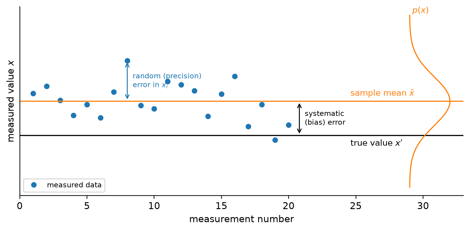
Measurement errors (such as the ones you saw during the last activity) enter through every stage of a monitoring system. Through sensors, we collect information about the physical asset or process. But like all measurements, they are only estimates of the true value of the attributes corresponding to the physical quantity in question. Given that we usually do not have access to the true value of the attribute, understanding the error from just one single measurement without any other truth reference is typically not possible. Instead, it is more useful to understand measurement errors by describing the properties of multiple repeated measurements, and/or comparing single measurements with other more trusted ones. Figure 8.1 illustrates both of these notions together.
Figure 8.1: Distribution of errors upon repeated measurements. Twenty readings of the same quantity under fixed conditions (dots) scatter about their sample mean \(\bar{x}\); the width of that scatter is the random (precision) error, and its probability density is sketched at the right. The sample mean itself sits a fixed distance from the true value \(x'\): that offset is the systematic (bias) error, and no amount of repetition reveals it.
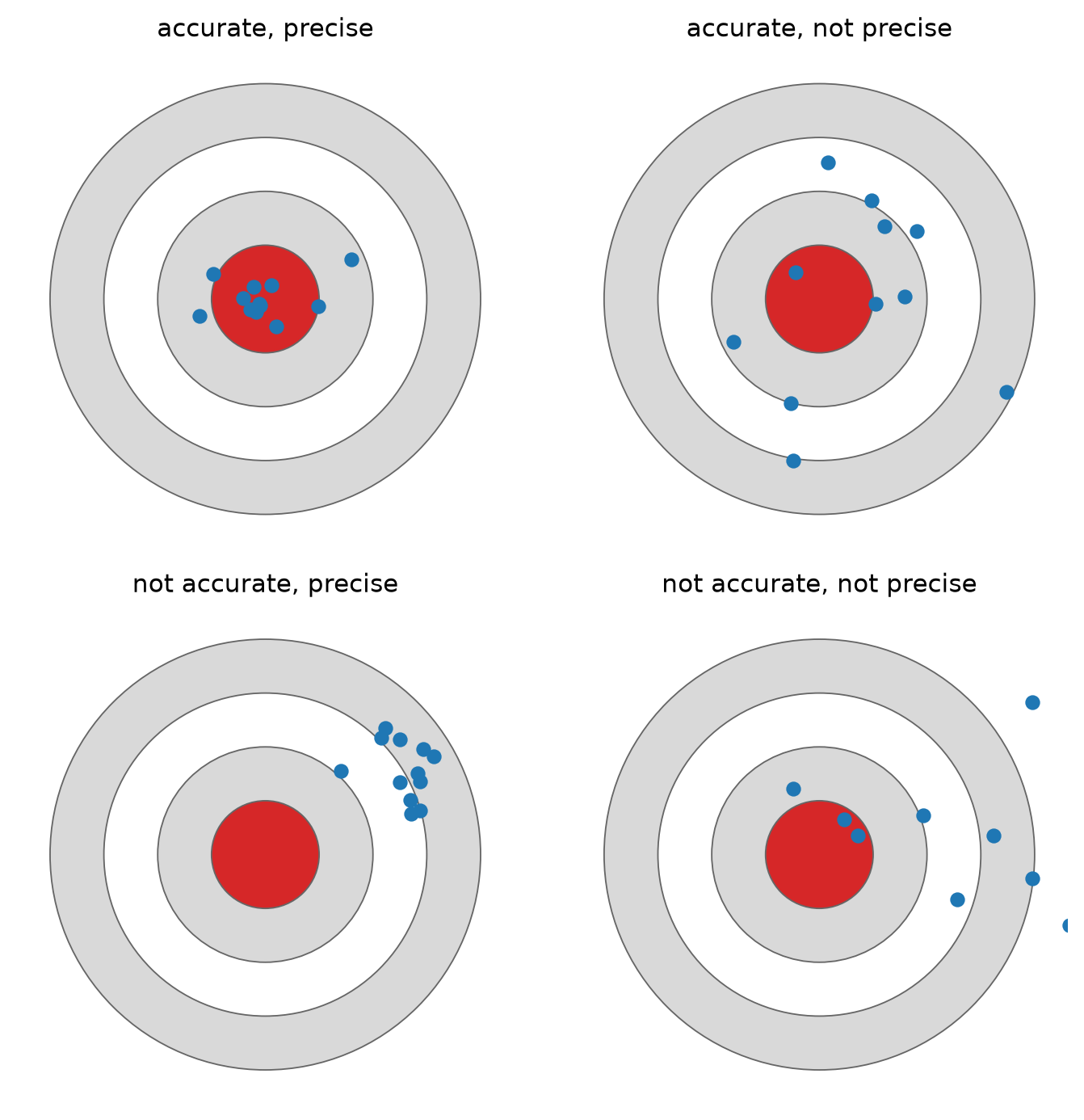
From this figure, it is easy to see that there are two kinds of errors. The first, which describes the spread of the repeated measurements around an average value, is the random error, and the quantity that characterizes it is often called the aleatory uncertainty. The second appears as a consistent deviation between all measurements and the true value (a constant difference). This is the systematic error, and the quantity that characterizes it is often called the epistemic uncertainty. Two other words belong here. Precision is the closeness of repeated readings to each other, so a precise instrument has small random error. Accuracy is the closeness of a reading to the true value, and an accurate instrument needs both errors to be small: a precise but biased instrument is like a rifle that groups its shots tightly a hand’s width from the bull’s-eye (Figure 8.2).
Figure 8.2: Accuracy and precision are different properties. Each panel shows twelve shots at the same target. Precision is the tightness of the group (left column vs. right column); accuracy is how close the group’s center is to the bull’s-eye (top row vs. bottom row). Only the top-left shooter is accurate, and only calibration — not more shots — can move the bottom-left group onto the target.
The vocabulary varies by field, and you will meet all of it, so Table 8.1 lines it up once. This chapter uses the first column, which is the one the Guide to the Expression of Uncertainty in Measurement (the GUM) uses (Joint Committee for Guides in Metrology 2008a).
Table 8.1: Three vocabularies for the same two errors.
To understand the random error, let’s assume for a moment that the true value of the attribute we are measuring is \(x'\). Let’s further assume that though we still do not have access to this value, we know the distribution of all possible values that a measurement of \(x'\) can result in (i.e., we have the probability density function for the population). In the case that there are no systematic errors, then simply computing the mean value of \(x\) over the population would give us \(x'\). In other words, since there is no systematic bias, and we can fully characterize the spread of the measurements around the true value, then the population mean should be equal to the true value. No assumption about the shape of the distribution is needed for that statement; “no systematic error” and “population mean equals the true value” are the same sentence. Shape starts to matter only when we write the uncertainty as a symmetric interval about the mean, as we are about to do, which is natural for a symmetric distribution and a rough summary for a skewed one.
But what happens if we do not have access to the population distribution, and the population is so large that we cannot reasonably sample all of the elements of it? Then we are left with finite samples from the population (e.g., a finite set of measurements) and we need to extrapolate population statistics from this sample. Thankfully, not all hope is lost. Under mild assumptions (e.g., errors are uncorrelated and follow a normal distribution) we can still formally characterize this relationship between sample statistics and the true value of the characteristic we are measuring. In particular, we can write down the following expression:
\[x' = \bar{x} \pm u_x \quad (P\%) \tag{8.1}\]
Here, \(\bar{x}\) represents the sample mean, and \(u_x\) represents the uncertainty on the measurements \(x\) caused by all types of errors combined. The \(P\%\) at the end indicates that this interval (from \(\bar{x} - u_x\) to \(\bar{x} + u_x\)), where we expect \(x'\) to be, is only true \(P\%\) of the times. In other words, the interval traps the true value with \(P\%\) probability. Every uncertainty statement in this lecture is a version of Equation 8.1, and the rest of the lecture is about building \(u_x\) honestly: from the scatter you can see, from the specifications you can read, and from the way errors travel through the formulas you apply.
TipActive Learning: Random and systematic, from your own readings
Using the measurements you collected for the crack length in the previous activity, try to estimate the value of the random and systematic uncertainty. Remember that there is a true value \(x'\) for the length of this crack. However, your measurements \(x_i\), \(i \in \{1, \dots, N\}\), have errors in them. Part of those errors is systematic (i.e., a constant bias always present in your measurements), while another part of it is random (e.g., it can be different from measurement to measurement due to experimental conditions and other factors).
Start by computing the random uncertainty. How would you characterize the spread of the measurements you took (i.e., how far away they are from the sample mean)? What statistical quantity would help you represent that spread?
Then try to compute the systematic uncertainty. How would you go about doing this? Do you need any additional information to answer this? Why or why not?
TipAnswer
Random part. The spread of your \(N\) readings about their mean is the sample standard deviation \(s\); it describes how far one more reading would typically fall from the mean. The uncertainty of the mean itself is smaller, \(s/\sqrt{N}\), which is why repeating a measurement helps. With four readings, \(s\) is a rough number and Section 8.7 will show how Student’s \(t\) accounts for that. In the web version, the summary below is computed from the readings you actually took.
crackStats = {const v = crackReadings.map(r => r.mm);if (v.length<2) returnhtml`<em>Take at least two readings with the ruler above and the summary appears here.</em>`;const n = v.length, mean = v.reduce((a, b) => a + b,0) / n;const s =Math.sqrt(v.reduce((a, b) => a + (b - mean) **2,0) / (n -1));returnhtml`<table style="font-size:0.9em"><tr><td>readings $N$</td><td>${n}</td></tr> <tr><td>sample mean $\\bar{x}$</td><td>${mean.toFixed(1)} mm</td></tr> <tr><td>sample standard deviation $s$</td><td>${s.toFixed(2)} mm</td></tr> <tr><td>standard deviation of the mean $s/\\sqrt{N}$</td><td>${(s /Math.sqrt(n)).toFixed(2)} mm</td></tr></table>`;}
Systematic part. Nothing in the scatter can reveal it. If the ruler’s conversion factor is wrong, every reading is wrong by the same percentage, the mean included, and the four readings agree with each other as well as ever. To estimate the bias you need something whose true value you trust: a reference. The image carries one, the bar marked 100 mm. Measure it with the same ruler. If the ruler reports 105 mm for it, the ruler reads about 5% high, and so do your crack readings; correcting them by that factor is a calibration, the subject of Section 8.4. Without a reference you can only bound the bias from what you know about the instrument, which is what Section 8.5.2 will call a Type B evaluation.
CautionConcept Check: Agreement is not accuracy
Your four ruler readings of the crack agree to within 0.5 mm. A colleague concludes that the crack length is known to 0.5 mm. What is wrong with that conclusion?
TipAnswer
The agreement bounds the random error only. A wrong conversion factor, a wrong choice of where the crack “ends”, or a camera that was not square to the wall would shift all four readings together and leave their agreement untouched. The 0.5 mm is a statement about precision; accuracy needs a reference or a bound on the systematic error as well.
8.3 Where Noise Comes From
As we saw before, errors can be categorized into systematic and random. We can think of systematic errors as a constant offset from the true value that shows up in any measurement we make with an instrument. For example, if the virtual ruler we used in the first activity had the wrong scale (i.e., the value used to convert from pixels to real distance was wrong), then all the measurements that we made with it would be consistently off by the same amount. Similarly, we can think of random errors as those that change with each measurement despite experimental conditions being fixed. The fact that it is difficult for your body to position the mouse cursor consistently at the same spot in repeated measurements causes measurements to vary despite the image of the wall being exactly the same in every turn.
To decide how much confidence to place in a measurement, we need an accounting of all the mechanisms that could affect it. An uncertainty budget is that accounting in a table: each row identifies an uncertain input, the evidence and assumptions used to quantify its uncertainty, and its contribution to uncertainty in the final result. For the photoresistor resistance, for example, the rows include repeated-reading scatter, fixed-resistor tolerance, and voltage-conversion uncertainty. The budget lets us combine these contributions and identify which improvement would matter most.
A budget is only as complete as the mechanisms we include. Figliola and Beasley organize the search into three groups, named after the three steps of any measurement: calibration, data acquisition, and data reduction (Figliola and Beasley 2019, §“Error Sources”). The grouping is bookkeeping, not physics: an error filed under the wrong heading changes nothing in the total, but an error that is never listed is missing from it. Let’s quickly review a subset of those sources:
8.3.0.1 Calibration errors
Suppose for a moment that we are conducting the same crack length measurements we were conducting during our first activity, but this time we are doing it on the physical wall (and not its digital picture). Just as we needed to have a way to convert the pixel distance to actual distance, with a real ruler or measurement tape we would need to have a way to convert the length of the instrument (ruler, tape) into a standardized value of length that we recognize (e.g., meters). The process that one follows to learn about this relationship is called calibration. In the case of a ruler, for instance, when the physical ruler was created (say, a metal sheet was cut into the shape of a ruler) we calibrate it by establishing a relationship between its length (or sub-portions of its length) and standard length measurements such as meters or inches. We thus create a mapping between the instrument’s output (the part of the ruler up to which a length is being measured) and the true value of that measurement (the length in units of meters/inches that it represents). This is what the ruler’s physical markers are expressing.
This calibration process, however, can introduce errors. Here are some ways this could happen:
The template you used to print the markers on the ruler is itself inaccurate.
You printed accurate markers on the ruler but forgot to take into account that the material the ruler is made of is very sensitive to temperature, and thus the length of the ruler will effectively change once you leave the cold room conditions you printed it at.
Any such errors that take place during calibration are then passed on to the subsequent measurements. Notice the chain hiding in the first bullet: the template was itself checked against something, which was checked against something else, up to a national standard. Every link carries its own uncertainty, and a calibration can never make an instrument better than the standard it was compared against.
8.3.0.2 Data acquisition errors
Even if the calibration errors we explored in the previous section are minimal, the process of acquiring measurements using the instrument is responsible for many other common sources of errors. For example, if during the measurement of the crack length we orient the ruler in a way that is not exactly parallel to the line that best represents its true length, then we introduce errors. More likely, we are prone to mis-attribute the starting and ending points for the length of the crack. Maybe the measurement was affected by operational conditions such as temperature (affecting the length of the ruler or the opening of the crack). There are many other similar problems, but all of these are catalogued under data acquisition errors. Every stage of the measurement chain from Lecture 2 contributes its own: the sensing element, the signal conditioning, the converter, and the environment they sit in.
8.3.0.3 Data reduction errors
Let’s now extend the story of the crack measurement by assuming that the estimated crack length would then be used to provide an estimate of the remaining useful life of the wall. Suppose there is an empirical function relating multiple consecutive crack length measurements over a period of 1 week to the remaining useful life. We can now say that our measurements are directly estimating the remaining useful life (once we apply this function). However, since the function is likely not perfect, any errors it contains will be present in our measurements of remaining useful life. Any such types of errors brought about by mapping instrument measurements to other quantities are catalogued under data reduction errors. A calibration curve fitted to too few points, a lookup table interpolated too coarsely, and a formula applied outside the range it was derived for all belong here.
8.3.1 Design-Stage Uncertainty
Different error sources work together to corrupt our measurements and affect the size of the interval represented in Equation 8.1. Thus, to really understand how good our measurements are (or will be) using Equation 8.1, we need to be able to do two things: (a) combine any information we have about the uncertainty brought about by each one of the error sources (i.e., calculate \(u_x\) with all the available information) and (b) compute the sample average with any available measurements.
The second part of this (computing the sample average) is very simple if measurements are available and unnecessary if all we want to know is how small of an interval around this value we will be able to construct to trap our true measurements. During the design stage of your instrument (i.e., when we are still deciding what instruments to use to capture the physical system) there are no actual measurements available. Thus, at this stage, we are only concerned with computing \(u_x\) and understanding how the different instrument choices affect this value.
Figliola and Beasley give this stage a two-line recipe (Figliola and Beasley 2019, §“Design-Stage Uncertainty Analysis”). The first line is the zero-order uncertainty: even a perfect instrument cannot report finer than its resolution, so
is the least uncertainty any reading of it can carry. The second line is the instrument uncertainty\(u_c\), assembled from the catalog’s error terms (linearity, hysteresis, repeatability, gain tolerance) by the root-sum-square (RSS) rule that the rest of this lecture will justify,
and the design-stage uncertainty of one instrument is \(u_d = \sqrt{u_0^2 + u_c^2}\). A chain of instruments combines its \(u_d\)’s the same way, once they are all expressed in the same units. The recipe’s value is not the number it produces, which is a floor rather than a forecast, but the comparison it forces: which link of the chain sets the floor?
Take the ADXL335 read by the ESP32’s 12-bit, 3.3 V converter, at a nominal reading of 1 g. The converter’s step is \(Q = 3.3\ \mathrm{V}/4096 = 0.806\) mV, so \(u_0 = 0.403\) mV, which at 300 mV/g is 1.3 mg. The sensor’s catalog terms, from the datasheet numbers already used in Lecture 2, are a nonlinearity of \(\pm 0.3\%\) of full scale (18 mg over the \(\pm 3\) g span) and a sensitivity tolerance of \(\pm 10\%\) (100 mg at 1 g). The converter has a catalog term of its own that is easy to overlook: Espressif documents that the ESP32’s internal reference, nominally 1100 mV, ranges from 1000 to 1200 mV from chip to chip, a gain error of up to \(\pm 9\%\) on every reading unless the chip is calibrated, which is 90 mg of the 1 g signal once the zero-g reading has been subtracted. Table 8.2 collects the terms.
Table 8.2: Design-stage terms for an ADXL335 on the ESP32 converter, at a 1 g reading.
Term
Value at 1 g
Kind
Removable by calibration?
ADXL335 sensitivity tolerance, \(\pm 10\%\)
100 mg
systematic
yes (one reference point)
ESP32 ADC reference spread, \(\pm 9\%\)
90 mg
systematic
yes (chip calibration or a known voltage)
ADXL335 nonlinearity, \(\pm 0.3\%\) FS
18 mg
systematic, but varies with input
only with a multi-point curve
ADC resolution, \(u_0 = Q/2\)
1.3 mg
random
no
Straight out of the box the RSS of the four terms is 136 mg, dominated by the two gain errors; with both gains calibrated out it is 18 mg, set entirely by the sensor’s nonlinearity. The 1.3 mg of converter resolution never matters in either case. That is the lesson Figliola and Beasley draw from their own voltmeter-and-transducer example: buying a finer converter would change nothing here, and a single calibration point changes almost everything. Resolution and accuracy are different specifications, which Assignment 1 asked you to explain and which Table 8.2 now shows in numbers.
8.3.2 Example Error Sources
Three sources recur in every electronic measurement chain, and this course has already met two of them. Each one below is classified as random or systematic, because that decides what can be done about it: random errors shrink with averaging, systematic errors do not.
Thermal noise. Every resistor is a noise source: the thermal agitation of its charge carriers produces a fluctuating voltage across its terminals even with nothing connected, with an rms value of
where \(k_B\) is Boltzmann’s constant, \(T\) the absolute temperature, \(R\) the resistance, and \(\Delta f\) the bandwidth over which the voltage is observed. It is random, white, and Gaussian, and it sets the floor below which no amplifier can help. The numbers put it in its place for the hardware of this course: the 10 kΩ divider resistor of Assignment 1 at 300 K, observed over a 100 Hz bandwidth, produces 0.13 µV rms; the GL5528 in the dark, at 1 MΩ, produces 1.3 µV; both are hundreds of times below the converter’s 0.8 mV step. Thermal noise matters when the source resistance is high, the bandwidth is wide, and the signal is small, which is the situation of a strain-gauge bridge feeding a high-gain amplifier, not of a divider feeding a 12-bit converter. Mitigation: lower resistances where the circuit allows, the narrowest bandwidth that passes the signal (Lecture 5’s low-pass filter does double duty), and averaging, which divides the rms by \(\sqrt{N}\).
Interference. Signals from elsewhere couple into the measurement: 60 Hz hum from mains wiring, switching transients from a motor drive, the ground-loop current of Lecture 5 flowing through a shared return. Over a long record interference looks random, but at any instant it is a deterministic addition, and its average over a record that is not a whole number of hum cycles does not vanish. The remedies were the subject of Lecture 5 and are only listed here: differential inputs and instrumentation amplifiers for what is common to both leads, shielding and twisted pairs for what is picked up along the way, a single ground point for what flows through the return, filtering for what lies outside the signal band, and synchronous averaging for what is periodic and known.
Quantization. The converter reports the nearest of \(2^n\) levels, so every sample carries an error between \(-Q/2\) and \(+Q/2\) (Lecture 4). For a signal that moves by many steps between samples the error is as good as random and uniformly distributed over that interval, and a uniform distribution of half-width \(a\) has standard deviation \(a/\sqrt{3}\), so the quantization error has
which for the ESP32 is 0.23 mV, against the 0.40 mV bound of Equation 8.2. The \(a/\sqrt{3}\) rule is not specific to converters: it is how the GUM converts any “somewhere between \(\pm a\)” statement into a standard uncertainty (Joint Committee for Guides in Metrology 2008a, sec. 4.3.7), and Section 8.5.2 uses it again. For a signal that sits still, quantization stops being random: a constant input always rounds the same way, the error is a fixed offset of up to \(Q/2\), and averaging a thousand samples returns the same wrong code a thousand times. Dither, a deliberate small noise added before conversion, restores the randomness, and so does the thermal and interference noise that is usually there anyway.
Table 8.3: The recurring sources, and what averaging can and cannot do about them.
Source
Random or systematic?
Shrinks with averaging?
Mitigation
Group
Thermal noise
random
yes, as \(1/\sqrt{N}\)
lower \(R\), narrower \(\Delta f\)
data acquisition
Interference
deterministic, random-looking
only if not synchronous with sampling
differential input, shield, single ground, filter
data acquisition
Quantization
random if the signal moves, fixed if it does not
yes / no
more bits, gain before the converter, dither
data acquisition
Gain and offset tolerance
systematic
no
calibration
calibration
Curve-fit residual
systematic at each input
no
better model, more points
data reduction
CautionConcept Check: What averaging buys
You average 100 consecutive ADC readings of a steady voltage. Which of the following is divided by 10: the thermal-noise contribution, the reference-voltage gain error, the quantization error?
TipAnswer
Only the thermal noise, and the quantization error if the input is jittering by more than a step so that the rounding errors are effectively random. The gain error is the same on all 100 readings and survives the average untouched, as does the quantization offset of a truly steady input. Averaging attacks random error; systematic error is the job of calibration.
8.4 Calibration
The second activity ended on a hard fact: the scatter of your readings said nothing about the ruler’s scale, and only a reference bar could. Calibration is the general form of that move, and the claim of this section is that it is not a laboratory ritual but a statistics problem, the same one you will meet again as regression in the MODELS third of the course. Seen that way, “calibration reduces systematic error” stops being a slogan and becomes something you can compute, including how much systematic error is left.
8.4.1 Calibration as parameter estimation
An instrument’s transfer relation, in the language of Lecture 2, is a function from the measurand to the output. Write it with its parameters showing,
\[y_i = g(x_i;\,\theta) + \varepsilon_i,\qquad i = 1,\dots,N, \tag{8.6}\]
where \(x_i\) is the value of a reference (a standard whose value we trust), \(y_i\) is what the instrument reported for it, \(\theta\) collects the parameters (for a linear instrument, a gain \(k\) and an offset \(b\), so \(g = kx + b\)), and \(\varepsilon_i\) is the random error of that reading. Calibration is the estimation of \(\theta\) from the pairs \((x_i, y_i)\). Using the instrument afterwards is the inversion of \(g\) at the estimate: a reading \(y\) becomes the measurand estimate \(\hat{x} = g^{-1}(y;\,\hat\theta)\).
Which \(\hat\theta\)? If the \(\varepsilon_i\) are independent and Gaussian with standard deviation \(\sigma\), the probability of the data we saw, viewed as a function of the parameters, is the likelihood
and since the first term does not involve \(\theta\), maximizing \(\ln L\) is the same as minimizing the sum of squared residuals. Under Gaussian noise, least squares is the MLE. For the linear instrument the minimization has the closed form you may remember from statistics,
and, what matters for this lecture, the estimates come with uncertainties: with \(\sigma\) estimated from the residuals as \(s^2 = \sum_i (y_i - \hat{k}x_i - \hat{b})^2/(N-2)\),
These two numbers are what calibration leaves behind. Before calibrating, the gain was wrong by an unknown amount up to the datasheet tolerance, a systematic error; after calibrating, it is wrong by an amount whose standard deviation is \(u(\hat{k})\), which shrinks with more points, a wider spread of reference values, and a quieter instrument. Calibration converts a systematic error into a smaller, quantified uncertainty of the estimated parameters, and Section 8.6 shows how that uncertainty travels into every subsequent reading through \(g^{-1}\).
The two-point calibration everyone has done, reading the instrument at two known values and drawing the line through them, is the case \(N = 2\) of Equation 8.9: the line passes through both points exactly, the residuals are zero, and \(N - 2 = 0\) degrees of freedom are left to estimate \(s\) from. The estimate is legitimate, but it carries no internal evidence of its own quality; the uncertainty of \(\hat{k}\) then has to come from what you know about the instrument’s noise rather than from the fit. A one-point calibration (one reference, gain assumed from the datasheet, offset adjusted) is the case \(N = 1\), where the data cannot separate \(k\) from \(b\) at all: something else must supply one of them, and the next subsection makes that “something else” explicit.
8.4.2 The datasheet as a prior
Before you took a single calibration point you were not ignorant of \(\theta\). The GL5528’s sheet says its resistance at 10 lux lies between 8 and 20 kΩ and that its exponent is \(0.7 \pm 0.1\); the ADXL335’s says 300 mV/g within \(\pm 10\%\). In the language of Bayesian statistics that knowledge is a prior distribution \(p(\theta)\), and Bayes’ rule combines it with the likelihood into a posterior, \(p(\theta \mid \text{data}) \propto L(\theta)\,p(\theta)\). The maximum a posteriori (MAP) estimate is the peak of the posterior. For a Gaussian prior with mean \(\theta_0\) and covariance \(\Sigma_0\), taking logarithms as before gives
which is the least-squares objective plus a penalty for straying from the datasheet. When \(g\) is linear in \(\theta\), so that the model is \(y = X\theta + \varepsilon\) for a design matrix \(X\) whose rows are \((x_i, 1)\), the posterior is exactly Gaussian, with
Three things fall out of Equation 8.12. First, with many precise points the \(X^{\mathsf T}X/\sigma^2\) term dominates and the MAP estimate tends to the MLE: the data overrule the datasheet. Second, with no points it returns the prior: the datasheet is what you use when you have not calibrated, which is exactly what Table 8.2 did. Third, with one point the matrix \(X^{\mathsf T}X\) is singular, the least-squares problem has no unique answer, and yet Equation 8.12 is perfectly well-posed: the prior supplies the direction the data cannot, which is the formal content of “one-point calibration adjusts the offset and trusts the datasheet gain”. Recalibration is the same equation run again with last year’s posterior as this year’s prior, and drift is the reason that prior has to be widened before it is reused.
8.4.3 Worked example: calibrating a GL5528 against a lux meter
Assignment 1 left the light channel uncalibrated in lux, and its last question asked what it would take to fix that. Here is the answer, worked with simulated data. The GL5528’s sheet gives the law \(R = R_{10}\,(E/10\ \text{lux})^{-\gamma}\)(Senba Sensing Technology, n.d.). It is nonlinear in \(E\) but, after logarithms, linear in the parameters:
\[\ln R = \ln R_{10} - \gamma\,\ln\!\left(\frac{E}{10}\right), \tag{8.13}\]
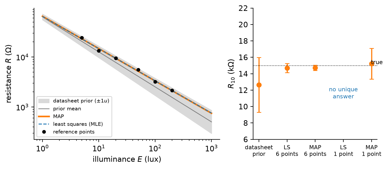
so with \(y = \ln R\), \(x = \ln(E/10)\), and \(\theta = (\ln R_{10}, -\gamma)\) it is the linear model of Equation 8.9. The prior comes from the sheet: \(R_{10}\) anywhere in 8 to 20 kΩ, which for \(\ln R_{10}\) is a uniform spread of half-width \(0.458\) about \(\ln(12.6\ \text{kΩ})\), hence a standard uncertainty of \(0.458/\sqrt{3} = 0.264\) by the rule of Equation 8.5; and \(\gamma = 0.7 \pm 0.1\), read the same way as a standard uncertainty of \(0.058\). The reference is a lux meter reading \(E\) at six illuminances between 5 and 200 lux while a bench ohmmeter reads \(R\). The simulated cell has \(R_{10} = 15\) kΩ and \(\gamma = 0.65\), both inside the sheet’s ranges, and every reading carries a few percent of noise.
Figure 8.3: Calibrating a GL5528 with six reference points (dots). Left: the datasheet alone (grey band: the spread of curves the prior allows, \(\pm 1\) standard uncertainty in each parameter), the least-squares fit to the data (dashed), and the MAP fit that combines the two (solid). Right: the same three answers for the parameter \(R_{10}\), with their standard uncertainties, and what happens with a single calibration point at 100 lux, where least squares cannot separate the two parameters and MAP still can.
Read the right panel from left to right. The datasheet alone allows \(R_{10}\) anywhere across its 8 to 20 kΩ range. Six points pin it down to a few percent, and the least-squares and MAP answers nearly coincide because six good points outweigh a vague prior. With a single point at 100 lux least squares has no answer at all, one equation for two unknowns, while MAP returns one: the point fixes the curve’s height where it was taken, the prior’s exponent carries it to other illuminances, and the posterior uncertainty is honest about that division of labor, wider than the six-point answer and narrower than the datasheet.
NoteOptional: What the framing hides
This callout is optional: it is not among the lecture’s learning objectives, and nothing after it depends on it. Read it before you calibrate something that matters.
The reference is not exact.Equation 8.6 treats \(x_i\) as known, and the lux meter has its own uncertainty. Ordinary least squares is the MLE only when that uncertainty is negligible against the instrument’s; when it is not, the model has errors in both variables and the estimator changes (Deming or total least squares). Metrology’s rule of thumb that the standard should be at least four times better than the instrument, a test uncertainty ratio of 4:1 or more, is precisely the condition under which the simpler estimator is good enough.
Two ways round. We fitted \(y\) on \(x\) and then inverted \(g\) to use the instrument, the “classical” approach. One could instead regress \(x\) on \(y\) directly and skip the inversion. The two are not equivalent, the second is biased but can have a lower mean-square error inside the calibrated range, and which to prefer has a literature of its own (Osborne 1991).
Bayes and the GUM. The GUM’s Type B evaluations (Section 8.5.2) are priors under another name, and whether the GUM as a whole is coherent from a Bayesian point of view has been argued in the metrology journals (Kacker and Jones 2003; Elster 2014). For this course it is enough to notice that “datasheet plus data” is a posterior, and that the two views agree whenever the model is linear and the distributions Gaussian.
What stays systematic.Equation 8.12 shrinks the uncertainty of \(\theta\), not the error of the model. If the real cell’s exponent changes with temperature and \(g\) has no temperature term, a thousand points taken at 20 °C leave that error exactly where it was, invisible in the residuals and present in every reading taken at 30 °C. Calibration reduces the systematic error you modeled; misspecification is the systematic error you did not.
CautionConcept Check: A thousand points
You calibrate a pressure transducer with a thousand reference points, all taken at 20 °C, and the fit’s parameter uncertainties are tiny. In service the transducer sits outdoors at 35 °C. Which part of its error did the thousand points reduce, and which part did they not touch?
TipAnswer
They reduced the uncertainty of the gain and offset at 20 °C almost to nothing. The temperature coefficient never appeared in the model, so the points carry no information about it; the systematic error at 35 °C is whatever the coefficient times 15 °C amounts to, and only a calibration that varies temperature, or a datasheet bound on the coefficient (a Type B term), can say how large it is.
8.5 Quantifying Uncertainty
Calibration handed us its uncertainties from a fit, but most of the numbers in an uncertainty budget come from humbler places: a column of repeated readings, or a line on a datasheet. The GUM sorts every component by where its number came from, and that sorting, rather than the random-versus-systematic one, is what decides how the number is computed (Joint Committee for Guides in Metrology 2008a, sec. 4).
The framing of Section 8.4 carries over. A measurement result is an estimate of the measurand, produced by an estimator (the sample mean, a fitted parameter, a formula applied to readings), and its uncertainty is a statement about the distribution of that estimator. The sample mean \(\bar{x}\) of \(N\) readings estimates the population mean; if the readings are independent with standard deviation \(\sigma\), the mean has standard deviation \(\sigma/\sqrt{N}\), and that is the number an uncertainty statement about \(\bar{x}\) is built on. Everything else is about how we get at \(\sigma\), or at the corresponding spread of something we never repeated.
8.5.1 Type A: repeated observations
A Type A evaluation obtains a standard uncertainty by statistical analysis of a series of observations. Given \(N\) readings \(x_1, \dots, x_N\) under fixed conditions, the sample standard deviation
estimates \(\sigma\), the scatter of one reading, and the standard uncertainty of the mean is
\[u_A(\bar{x}) = \frac{s}{\sqrt{N}}, \tag{8.15}\]
with \(\nu = N - 1\)degrees of freedom, a number that will matter in Section 8.7 because \(s\) from four readings is a far rougher estimate of \(\sigma\) than \(s\) from a hundred. This is the quantity Figliola and Beasley call the precision index of the mean, and it is what “repeatability” means once a number is attached to it.
The case-study log, data/light_channel_synthetic.csv, is a simulated record in the format of the Assignment 1 logger (one row every 250 ms, four illumination conditions, each recorded three times for 24 s; the numbers are generated, not measured, and Section 8.8 says how). Its first “ambient” trial gives a concrete Type A evaluation:
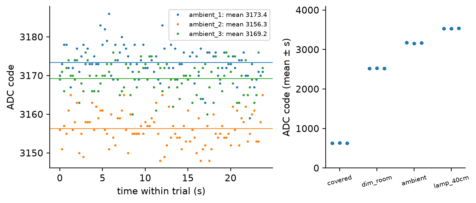
N = 96, mean = 3173.4 codes, s = 4.25 codes, u_A(mean) = s/sqrt(N) = 0.43 codes
Ninety-six readings scatter by about four codes, and their mean is known to under half a code. That half-code is the uncertainty of the mean of this trial; it says nothing about whether a second trial under “the same” conditions would land on the same mean, which is a different question that the case study takes up.
8.5.2 Type B: specifications and prior knowledge
A Type B evaluation obtains a standard uncertainty by any means other than the statistics of repeated observations: a manufacturer’s specification, a calibration certificate, a handbook value, a physical bound, or experience with the instrument. The number still has to be a standard uncertainty, a standard deviation, so each source statement is converted according to what it claims:
“Within \(\pm a\)”, nothing more said. Take the value as equally likely anywhere in the interval: a rectangular distribution, standard uncertainty \(a/\sqrt{3}\) (Equation 8.5). The ESP32 reference spread of \(\pm 9.1\%\) becomes \(u = 5.25\%\); a 5% resistor becomes \(2.9\%\); a 3.3 V regulator specified to \(\pm 2\%\) becomes \(1.2\%\).
“Within \(\pm a\)”, values near the center more likely. A triangular distribution, \(a/\sqrt{6}\). Appropriate when the bound is a loose one that is rarely approached.
“\(\pm U\) at 95% confidence”, as on a calibration certificate. Divide by the coverage factor, \(u = U/2\) for a normal distribution at 95%. A certificate reading “\(\pm 0.05\) °C (95%)” contributes \(0.025\) °C.
A noise density, such as the ADXL335’s \(150\ \mu\text{g}/\sqrt{\text{Hz}}\). Multiply by the square root of the bandwidth: \(u = 150 \times \sqrt{100} = 1.5\) mg over 100 Hz. This is a random effect, and it is nonetheless evaluated Type B, because the number came from a sheet and not from your own readings.
That last bullet is the point the older vocabulary blurs. Figliola and Beasley’s edition on my shelf says that an error should be treated as a precision error “if it can be statistically estimated in some manner; otherwise treat the error as a bias error” (Figliola and Beasley 2019, §“Bias and Precision Errors”), which equates how it was evaluated with what kind of effect it is. The two questions usually have the same answer, which is why the shortcut survives, but they are different questions. A systematic effect can be evaluated Type A: calibrate against a standard ten times and the scatter of the ten offsets is a statistical estimate of a bias. A random effect can be evaluated Type B: the noise density above. Table 8.4 gives one example of each combination. This chapter keeps the two classifications apart: random or systematic decides whether averaging helps and whether calibration can remove it; Type A or Type B decides which formula produces the number.
Table 8.4: The two classifications are independent: one example in each cell.
Type A (from your repeated readings)
Type B (from other knowledge)
Random effect
scatter of 96 ADC codes in one trial, \(s/\sqrt{N}\)
noise density on the ADXL335 sheet, \(150\ \mu\text{g}/\sqrt{\text{Hz}}\)
Systematic effect
ten repeated comparisons against a reference lux meter, scatter of the offsets
ESP32 reference spread, \(\pm 9\%\) rectangular
CautionConcept Check: Sort the budget
For the Assignment 1 light channel, classify each component as random or systematic, and as Type A or Type B: (a) the scatter of codes within a 24 s trial; (b) the 5% tolerance of the 10 kΩ resistor; (c) the ESP32 reference spread; (d) the change in mean code between three repeats of the same condition; (e) the quantization step; (f) the GL5528’s \(\gamma\) read off the datasheet.
TipAnswer
random, Type A. (b) systematic for this one board, Type B. (c) systematic for this chip, Type B unless you measure it against a known voltage, which makes it Type A. (d) it looks like scatter but is a reproducibility effect between repeats: random over many repeats, Type A from the three means. (e) random if the input jitters, Type B from \(Q/\sqrt{12}\). (f) systematic for this cell, Type B from the sheet’s \(\pm 0.1\), until a calibration (Type A) replaces it.
8.6 Propagating Uncertainty
Sometimes, the measurements we make are just the means to an end because what we are interested in is not the measured quantity itself but some function of the measurement(s). In these cases, it becomes important to evaluate the impact that the uncertainty can have on the output of this function we are going to be calculating. In other words, we want to understand how sensitive the output of this function (which could be a complex mathematical model, a decision-making process, a simulation, etc.) is to the uncertainty we have for each of its inputs.
Consider, for instance, a cantilever beam of length \(L\), subject to a point load \(P\) located at a distance \(a\) from the fixed end of the beam. Imagine that we are interested in the total deflection of the beam, but cannot directly measure it. Instead, we rely on our engineering knowledge from statics and use the formula for deflection after measuring the length of the beam, the distance of the point load, the magnitude of the point load, and getting an elastic modulus \(E\) for the material from a table. Let’s assume that the beam has a second moment of area \(I\) and that we do not have any uncertainty about that (the cross-section dimensions are perfectly measured).
Using this, the deflection \(\delta\) at the end of the beam (its maximum deflection) is given by the following formula:
However, due to various measurement uncertainties, the following parameters are not known exactly:
The length of the beam \(L\) has an uncertainty of \(u_L\)
The distance \(a\) from the fixed end where the load is applied has an uncertainty of \(u_a\)
The magnitude of the point load \(P\) has an uncertainty of \(u_P\)
The elastic modulus \(E\) of the beam has an uncertainty of \(u_E\)
How do these uncertainties propagate to the resulting value of deflection?
Start from what a small change in each input does to the output. For inputs close to their nominal values, \(\delta\) is well approximated by the first-order terms of its Taylor expansion, so a change \(\Delta L\) produces a change \((\partial\delta/\partial L)\,\Delta L\) in the deflection, and likewise for the other three. The partial derivatives are the sensitivities: they say how much each input’s error is amplified or attenuated on its way to the result. If every input happened to err in the direction that pushes \(\delta\) the same way, the errors would simply add, and the uncertainty in the deflection could be as large as
This is the worst-case bound, what Taylor calls the provisional rule (Taylor 1997, Ch. 3): it assumes the four errors conspire, which independent errors do not. If instead the uncertainties in the input variables are independent of each other (i.e., there is no covariance between the variables), their contributions add the way independent random variables do, in variance, and the expression for the propagation of uncertainty becomes
the root-sum-square again, which is never larger than Equation 8.17 and usually much smaller. Both expressions rest on the same linearization, and both are valid only when the uncertainties are small enough that the higher-order terms of the expansion are negligible, a condition Section 8.6.1 makes visible. What separates them is not accuracy but the assumption about how the errors combine, and Equation 8.18 is the one to report unless you have a reason to believe the errors are correlated.1
TipActive Learning: Where the uncertainty comes from
Let’s assume that we have specific values for the parameters of this beam deflection problem we have been considering:
\(L = 5\) m, with \(u_L = 0.01\) m
\(a = 2.5\) m, with \(u_a = 0.02\) m
\(P = 1000\) N, with \(u_P = 50\) N
\(E = 200 \times 10^9\) Pa, with \(u_E = 5 \times 10^9\) Pa
\(I = 0.001\ \text{m}^4\)
Estimate the contribution of each uncertainty.
Calculate the partial derivatives \(\frac{\partial \delta}{\partial L}\), \(\frac{\partial \delta}{\partial a}\), \(\frac{\partial \delta}{\partial P}\), and \(\frac{\partial \delta}{\partial E}\).
Using the above values for \(L\), \(a\), \(P\), \(E\), and their respective uncertainties \(u_L\), \(u_a\), \(u_P\), \(u_E\), calculate how each uncertainty contributes to the overall uncertainty \(u_\delta\).
Interpretation.
Discuss which parameter’s uncertainty has the largest influence on the uncertainty in the deflection \(\delta\), and why.
Suggest how one could minimize the overall uncertainty in the deflection calculation. For example, would it make sense to invest in more precise measurements of one variable over another?
TipAnswer
The nominal deflection is \(\delta = 0.0651\) mm. Each derivative is easiest in relative form, since \(\delta\) is a product of powers of its inputs except for the factor \((3L - a)\):
Combined by Equation 8.18, \(u_\delta = 3.8 \times 10^{-6}\) m, or 5.8% of \(\delta\); the worst case of Equation 8.17 would be 9.2%. The load dominates: its 5% uncertainty enters at full strength because \(\delta\) is proportional to \(P\), and the modulus is next for the same reason. Measuring the beam’s length ten times better would change the answer by nothing visible, because \(L\) enters only through \((3L - a)\) and a 0.2% error there is 0.24% of the result. The investment goes into the load cell, then the modulus (a coupon test instead of a table), and the tape measure stays where it is.
The general lesson: rank the contributions before improving anything, and stop improving a term once it is well below the largest. This ranking is a design tool, and the same table for the Assignment 1 channel is the heart of the case study.
8.6.1 Formalizing the Propagation
The beam had four inputs and a formula we could differentiate by hand. The general problem is one input and a curve, and Figliola and Beasley’s picture of it (Figliola and Beasley 2019, §“Uncertainty Analysis: Error Propagation”) is worth carrying around, because it shows both what linearization does and when it fails.
Let \(y = f(x)\) relate a measured variable \(x\) to a result \(y\), and suppose the measurement has put \(x\) within \(\bar{x} \pm u_x\). Expanding \(f\) about the operating point \(\bar{x}\),
The first term is the nominal result, the second maps the uncertainty band in \(x\) onto a band in \(y\) through the slope, and the remaining terms are what the first-order rule throws away. Keeping only the slope gives
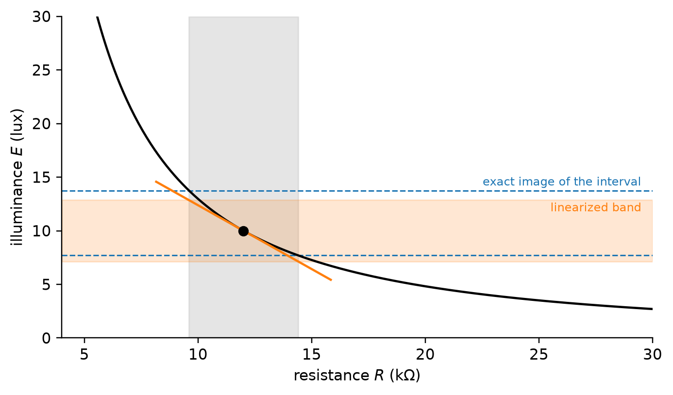
which is exact for a straight line and an approximation for anything else, good when the curve is nearly straight across the width of the band and poor when it bends within it. The widget below draws exactly that picture for the GL5528’s illuminance law, \(E = 10\,(R/R_{10})^{-1/\gamma}\) lux, which bends hard: move the operating point down toward the dark end, or widen the band, and watch the tangent’s symmetric band drift away from the true, lopsided image of the interval.
viewof prop = Inputs.form({Rbar: Inputs.range([2,60], {value:12,step:0.5,label:"operating point R̄ (kΩ)"}),uRel: Inputs.range([1,40], {value:20,step:1,label:"uncertainty u_R (% of R̄)"}),})
Figure 8.4: Propagation through a curve, for the GL5528 law \(E = 10\,(R/R_{10})^{-1/\gamma}\) with \(R_{10} = 12\) k\(\Omega\) and \(\gamma = 0.7\), at an operating point of 12 k\(\Omega\) with a 20% uncertainty band (grey). The tangent at the operating point (orange) maps the band to a symmetric interval in \(E\) (orange band); the curve itself maps it to the lopsided interval between the dashed lines. The interactive version of this figure lets you move the operating point and widen the band.
Several inputs. For a result \(R = f(x_1, x_2, \dots, x_L)\) the expansion has one slope per input, the sensitivity coefficients
which is Equation 8.18 with the beam’s four names replaced by an index. It is the Kline and McClintock second-power relation (Kline and McClintock 1953; Holman 2011), the GUM’s law of propagation of uncertainty (Joint Committee for Guides in Metrology 2008a, sec. 5.1), and the reason the RSS rule appeared in Equation 8.3 before it was justified: combining elemental errors is propagation through a sum, where every \(\theta_i = 1\). Reported through Equation 8.1, the result is \(R' = \bar{R} \pm u_R\) with \(\bar{R} = f(\bar{x}_1, \dots, \bar{x}_L)\), and the terms \(\theta_i u_{x_i}\), ranked, are the budget.
The handout Propagation of Uncertainty derives Equation 8.22 in full. It shows that the result rests on two separate steps, each with its own assumption: replacing \(f\) by its tangent plane, the first-order Taylor expansion, which assumes \(f\) is nearly linear over the spread of the inputs; and computing the variance of the resulting linear combination, which reduces to the root-sum-square only when the inputs are uncorrelated. It then gives the general form for correlated inputs, the second-order corrections with worked examples of when first order fails, and the step from a propagated standard uncertainty back to a coverage interval.
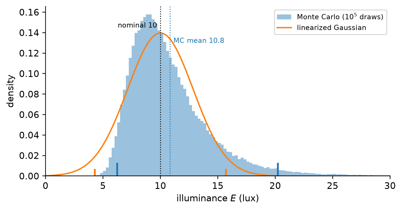
When it is exact, and when it is not. If \(f\) is linear and the inputs are independent and Gaussian, the result is a linear combination of independent Gaussians, which is itself Gaussian with exactly the variance of Equation 8.22: propagation is then not an approximation but a theorem, and a coverage interval for \(R\) follows from the normal distribution with no further assumption. Nonlinearity breaks both halves. The variance is only approximately Equation 8.22 (the second-order term of Equation 8.19 contributes), the mean of \(R\) shifts away from \(f(\bar{x})\), and the distribution of \(R\) is no longer Gaussian, so a symmetric \(\pm u_R\) interval misdescribes it, as the widget showed. The remedy that needs no derivatives at all is the Monte Carlo method of the GUM’s first supplement (Joint Committee for Guides in Metrology 2008b): draw the inputs from their distributions many times, evaluate \(f\) for each draw, and read the result’s mean, standard deviation, and coverage interval from the sample. Figure 8.5 does this for the widget’s default case.
Figure 8.5: Monte Carlo against linearization for the GL5528 law at \(\bar{R} = 12\) k\(\Omega\) with a Gaussian 20% uncertainty in \(R\). The histogram is \(10^5\) draws pushed through the curve; the orange curve is the Gaussian that first-order propagation predicts. The draws are skewed toward high illuminance, their mean sits at 10.8 lux rather than the nominal 10, their standard deviation is 36% larger than the first-order figure, and the 95% interval from the draws (blue ticks) reaches much further right than the symmetric \(\pm 2u\) interval (orange ticks).
NoteOptional: Sequential perturbation, when you cannot differentiate
This callout is optional: it is not among the lecture’s learning objectives, and nothing after it depends on it. It is the tool to reach for when \(f\) is a simulation, a spreadsheet, or a black box.
The sensitivities of Equation 8.21 do not need a formula for \(f\), only the ability to evaluate it. Figliola and Beasley’s sequential perturbation replaces each derivative with a finite difference: evaluate the result at the nominal inputs, \(R_0 = f(\bar{x}_1, \dots, \bar{x}_L)\); then, one input at a time, evaluate it with that input raised by its uncertainty, \(R_i^{+} = f(\dots, \bar{x}_i + u_{x_i}, \dots)\), and lowered, \(R_i^{-}\); take
For the beam it reproduces the analytic answer to three figures, and for a finite-element model of the same beam it would be the only option. Its limitation is the same as linearization’s: the step \(u_{x_i}\) must be small enough that \(f\) is nearly straight across it, and the averaging of the up and down steps in Equation 8.23 is a partial defense, not a cure.
CautionConcept Check: Spending the budget
For the beam, you can afford either a load cell twice as good (\(u_P\) halved) or a laser distance meter ten times as good as the tape (\(u_L\) divided by ten). Which reduces \(u_\delta\) more, and by roughly how much?
TipAnswer
Halving \(u_P\) takes the load’s contribution from 5.0% to 2.5% and \(u_\delta\) from 5.8% to about 3.8%. Dividing \(u_L\) by ten takes a 0.24% contribution to 0.02% and changes \(u_\delta\) in the third decimal. Contributions add in quadrature, so the largest one is the only one worth attacking, and a term below a third of the largest is already invisible.
8.7 Combining and Reporting
A budget is a list of standard uncertainties from Type A and Type B evaluations, each already multiplied by its sensitivity. The last two steps are to combine the list into one number and to state that number in a form that carries its own meaning: the width, the probability it claims, and what it covers.
8.7.1 Combining
For independent components the rule is the one we have used all along. The combined standard uncertainty is
with \(\theta_i = 1\) when the components are elemental errors in the measured quantity itself. Two conditions hide in it, and Figliola and Beasley are emphatic about the first (Figliola and Beasley 2019, §“Combining Elemental Errors: RSS Method”): every term must be expressed at the same probability level, which is why Section 8.5.2 insisted on converting each source statement to a standard uncertainty before it entered the list. Adding a “\(\pm\) 2%” that was a 95% bound to a “\(\pm\) 2%” that was a standard deviation produces a number that means nothing. The second condition is independence; correlated components need the cross terms of the footnote in Section 8.6.
8.7.2 Coverage
A standard uncertainty is one standard deviation. To turn it into an interval with a stated probability, multiply by a coverage factor\(k\): the expanded uncertainty is \(U = k\,u_c\), and the result is reported as \(x' = \bar{x} \pm U\). For a result whose distribution is close to normal, \(k = 2\) gives a level of confidence of about 95% and \(k = 3\) about 99.7%. The GUM’s default, and the convention of this course, is \(k = 2\) stated explicitly (Joint Committee for Guides in Metrology 2008a, sec. 6).
That default assumes \(u_c\) is well known. When the dominant component is a Type A evaluation from few readings, \(s\) is itself uncertain, and the factor that produces a 95% interval is larger than 2: it is the quantile of Student’s \(t\) distribution with \(\nu = N - 1\) degrees of freedom, \(t_{\nu,95}\). The numbers are worth remembering:
Table 8.5: The 95% coverage factor from Student’s \(t\), by number of readings.
\(N\) readings
2
3
4
5
10
30
100
\(\infty\)
\(t_{N-1,\,95}\)
12.71
4.30
3.18
2.78
2.26
2.05
1.98
1.96
Your four ruler readings are the case in point. With a standard deviation of, say, 1.2 mm, the standard uncertainty of their mean is \(1.2/\sqrt{4} = 0.6\) mm; \(k = 2\) would claim \(\pm 1.2\) mm at 95%, but three degrees of freedom warrant \(t_{3,95} = 3.18\) and the honest interval is \(\pm 1.9\) mm. Below about ten readings, use \(t\); above thirty, \(k = 2\) is close enough.
Where the \(t\) factor comes from is worth seeing once. The handout From Measurement Uncertainty to Confidence Intervals starts from a statement of the form \(x_{\text{true}} = \bar{x} \pm u_x\) with a stated probability and derives the interval in two stages. When \(\sigma\) is known, the error of the mean divided by \(\sigma/\sqrt{N}\) is standard normal, and the factor is the normal quantile, 1.96 for 95%. When \(\sigma\) is replaced by the sample standard deviation of the same readings, that ratio follows Student’s \(t\) with \(N - 1\) degrees of freedom instead, which is why Table 8.5 is needed. The handout also explains what the stated probability does and does not promise, and why the interval accounts only for the random part of the error.
NoteOptional: Effective degrees of freedom
This callout is optional: it is not among the lecture’s learning objectives, and nothing after it depends on it. It answers the question “which \(t\)?” when a budget mixes few-reading Type A terms with Type B terms.
When \(u_c\) combines components with different degrees of freedom, the GUM’s Annex G assigns the combination an effective number by the Welch–Satterthwaite formula (Joint Committee for Guides in Metrology 2008a, sec. G.4),
with \(\nu_i = N_i - 1\) for a Type A term and \(\nu_i = \infty\) for a Type B term whose bound is taken as exact, so that Type B terms drop out of the denominator. The coverage factor is then \(t_{\nu_{\text{eff}},95}\). Example: a Type A term of 0.5 units from four readings (\(\nu = 3\)) combined with a Type B term of 0.4 units gives \(u_c = 0.64\), \(\nu_{\text{eff}} = 0.64^4 / (0.5^4/3) = 8.1\), and \(k = t_{8.1,95} = 2.30\) rather than the 3.18 the Type A term alone would demand or the 2 the Type B term alone would allow. Figliola and Beasley use the same formula, written for their precision indices, in their multiple-measurement procedure.
8.7.3 Systematic and random, together
The budgets in Figliola and Beasley keep the two kinds of error in separate columns until the very end: a bias limit\(B\), the RSS of the systematic estimates, each stated as a 95% bound, and a precision index\(P\), the RSS of the Type A standard deviations of the means, combined as
This is Equation 8.24 and a coverage factor in a different order of operations. Translate \(B\) into a standard uncertainty by dividing by its own coverage factor, \(u_B = B/2\), keep \(u_A = P\), and the GUM’s \(U = k\sqrt{u_A^2 + u_B^2}\) with \(k = 2\) reproduces Equation 8.26 except for the difference between \(t_{\nu,95}\) and 2, which the previous callout handles. The two conventions agree on the arithmetic; they differ on when the coverage factor is applied. This chapter applies it once, at the end, because that is how datasheets and calibration certificates expect to be read, and because it keeps a standard uncertainty, the quantity that propagates by Equation 8.22, distinct from an interval, the quantity that gets reported.
8.7.4 Reporting
A result without its uncertainty is not a measurement result, and an uncertainty without its coverage factor is not an uncertainty. Moffat’s advice on describing experimental results is four decades old and still the best short guide (Moffat 1988); the rules below are its core, in the GUM’s notation.
State the estimate and the expanded uncertainty with the coverage factor and the level it implies: “\(R_L = 2.94\ \text{kΩ} \pm 1.40\ \text{kΩ}\) (\(k = 2\), about 95%)”. “\(\pm 1.40\) kΩ” alone is ambiguous between one standard deviation and a 95% bound, a factor of two.
Round the uncertainty to one or two significant figures, and the estimate to the same decimal place. A deflection of 0.0651234 mm with an uncertainty of 0.008 mm is \(0.065 \pm 0.008\) mm; the trailing digits are noise dressed as information.
Say what the budget contains and under what conditions. Which components, Type A from how many readings, which Type B sources and their assumed distributions, at what temperature, with what calibration state. An interval that omits the systematic terms is a statement about repeatability and should say so.
Say how it was propagated when the model is nonlinear: first-order, or Monte Carlo with its two percentiles, which may be asymmetric and should then be reported as such (“\(2.93\ \text{kΩ}\), 95% interval 1.83 to 4.26 kΩ”).
Before and after, for the beam of Section 8.6: “\(\delta = 0.0651234\) mm \(\pm 0.004\) mm (probably)” becomes “\(\delta = 0.065 \pm 0.008\) mm (\(k = 2\)), by first-order propagation of the input uncertainties in the activity’s table, with \(I\) taken as exact; the load’s uncertainty accounts for three quarters of the variance.”
CautionConcept Check: Two identical-looking claims
Two reports of the same quantity read “\(12.30 \pm 0.05\) (\(k = 2\))” and “\(12.30 \pm 0.05\) (one standard deviation)”. Which is the stronger claim, and by how much?
TipAnswer
The first. It says the 95% interval is \(\pm 0.05\), so its standard uncertainty is \(0.025\); the second’s standard uncertainty is \(0.05\), twice as large, and its 95% interval would be \(\pm 0.10\). Same digits, a factor of two apart, which is why rule 1 exists.
8.8 Case Study: An Uncertainty Budget for the Assignment 1 Light Channel
Assignment 1 had you convert a median ADC code into a “nominal estimate” of the GL5528’s resistance and called it nominal for a reason. This case study attaches the missing uncertainty to that number, using every tool of the lecture in order, and finds that the answer is dominated by a term that twelve bits of resolution say nothing about.
The data. The log in data/light_channel_synthetic.csv is simulated: it was generated by a script, make_case_data.py, to look like a real Assignment 1 record (four conditions, three 24 s repeats each, one row every 250 ms, the starter firmware’s column names) with realistic noise, a per-repeat wobble in the illuminance, and one ADC gain error of the kind Espressif documents, whose value the analysis below is not told. The last point matters: it is exactly the situation on a real board. We analyze the “ambient” condition.
Figure 8.6: The three ambient-light trials of the simulated log (left), each 96 samples at 4 S/s: within a trial the codes scatter by about four counts, but the three trial means differ by up to seventeen. Right: mean and standard deviation of every trial in the log, showing the same pattern in every condition and, for the covered sensor, codes far from zero because the divider’s fixed resistor sets a floor.
Step 1, Type A. Two scatters are visible in Figure 8.6, and they are different quantities. Within a trial the codes have a pooled standard deviation of 4.1 counts; independent within-trial noise alone would contribute \(u = 4.1/\sqrt{288} = 0.24\) counts to the mean of all 288 ambient samples. Between the three trials the means are 3173.4, 3156.3, and 3169.2, a standard deviation of 8.9 counts, and the uncertainty of their average from that scatter is \(8.9/\sqrt{3} = 5.1\) counts, twenty times the within-trial term. That is the difference between repetition and replication that Figliola and Beasley build their higher-order uncertainties on (Figliola and Beasley 2019, §“Advanced-Stage and Single-Measurement Uncertainty Analysis”): repeating samples inside a trial measures the instrument’s noise; repeating the trial measures how well the condition was reproduced, and the second is what a claim about “ambient light” is actually subject to. The Type A term for the mean code is therefore 5.1 counts, or 0.16% of the grand mean of 3166.3. The scatter of the trial means already includes within-trial noise, so adding the 0.24-count contribution again would count that noise twice.
Step 2, Type B. From Section 8.5.2, each as a standard uncertainty, relative to the quantity it affects: the ESP32 reference spread, \(\pm 9.1\%\) rectangular, \(u = 5.25\%\) of \(V_{out}\); the 3.3 V supply, taken as \(\pm 2\%\), \(u = 1.15\%\); the fixed resistor, 5% tolerance, \(u = 2.89\%\); quantization, \(Q/\sqrt{12} = 0.29\) counts, or 0.009% of the reading, which is inside the observed scatter already and is listed only to show its size.
Step 3, propagate. The measurement model is the divider inverted, \(R_L = R_f\,(V_s/V_{out} - 1)\) with \(V_{out} = \text{code} \times Q\). Its relative sensitivities, \((\partial R_L/\partial x)(x/R_L)\), are \(-V_s/(V_s - V_{out})\) for \(V_{out}\), \(+V_s/(V_s - V_{out})\) for \(V_s\), and \(1\) for \(R_f\). At the ambient operating point, \(V_{out} = 2.551\) V, the first two are \(\mp 4.41\): a 1% error in the voltage becomes a 4.4% error in the resistance, because \(R_L\) depends on the small difference \(V_s - V_{out}\). The budget follows, each row a standard uncertainty times its sensitivity.
Show the code
cbar = amb.adc_code.mean(); means3 = amb.groupby("condition").adc_code.mean(); s_within = np.sqrt((amb.groupby("condition").adc_code.std(ddof=1)**2).mean())uA_within, uA_between = s_within / np.sqrt(amb.shape[0]), means3.std(ddof=1) / np.sqrt(3)uA_rel = uA_between / cbarV_out = cbar * Q; R_L = RF * (VS / V_out -1); sens_V = VS / (VS - V_out)budget = pd.DataFrame([ ("Type A: mean code (from trial means)", uA_rel *100, sens_V), ("quantization, $Q/\\sqrt{12}$ (already in scatter; not added)", Q / np.sqrt(12) / V_out *100, sens_V), ("ADC gain: reference spread $\\pm 9.1\\%$, rectangular", 100/1100/ np.sqrt(3) *100, sens_V), ("supply $V_s$: $\\pm 2\\%$, rectangular", 2/ np.sqrt(3), sens_V), ("fixed resistor $R_f$: $\\pm 5\\%$, rectangular", 5/ np.sqrt(3), 1.0),], columns=["component", "u_i (% of its quantity)", "relative sensitivity"])budget["contribution to R_L (%)"] = budget["u_i (% of its quantity)"] * budget["relative sensitivity"]u_c_rel = np.sqrt((budget.loc[[0, 2, 3, 4], "contribution to R_L (%)"]**2).sum())rows = [f"| {r.iloc[0]} | {r.iloc[1]:.2f} | {r.iloc[2]:.2f} | {r.iloc[3]:.2f} |"for _, r in budget.iterrows()]rows += [f"| **combined standard uncertainty $u_c$** | | | **{u_c_rel:.2f}** |", f"| **expanded uncertainty $U$ ($k = 2$)** | | | **{2* u_c_rel:.2f}** |"]print("| Component | $u_i$ (% of its quantity) | relative sensitivity | contribution to $R_L$ (%) |\n|---|---|---|---|\n"+"\n".join(rows)+"\n\n: Uncertainty budget for $R_L$ under the ambient condition, all rows as standard uncertainties. {#tbl-budget}")
Table 8.6: Uncertainty budget for \(R_L\) under the ambient condition, all rows as standard uncertainties.
Component
\(u_i\) (% of its quantity)
relative sensitivity
contribution to \(R_L\) (%)
Type A: mean code (from trial means)
0.16
4.41
0.72
quantization, \(Q/\sqrt{12}\) (already in scatter; not added)
by first-order propagation of the five components above, with the ADC uncalibrated. A Monte Carlo evaluation with the same inputs (the three Type B terms drawn from their rectangular distributions, the code from a normal one) gives a standard deviation of 24% and a 95% interval from 1.83 to 4.26 kΩ, wider on the high side because the inversion is convex; the first-order figure is a fair summary and the Monte Carlo interval is the one to quote if the asymmetry matters.
What the budget says. One row is 94% of the variance: the converter’s gain. The twelve-bit resolution that Assignment 1 computed so carefully contributes 0.04% of \(R_L\), and even the within-trial scatter, the thing repetition improves, is invisible next to the reproducibility of the condition. Two design decisions follow, and both are cheap. First, calibrate the converter: reading a known voltage once, or using the reference value Espressif burns into the chip, removes the dominant row and takes \(u_c\) from 23.9% to 5.9%. Second, move the operating point: the sensitivity of 4.4 comes from operating the divider near the top of its range for this cell, and a fixed resistor closer to \(R_L\) would put \(V_{out}\) near \(V_s/2\), where the sensitivity is 2, halving every voltage-side row. Assignment 1’s question about exchanging the two resistors was this question in disguise. And the closing check that only a simulation allows: the script that generated the log used a cell whose true resistance at this illuminance is 2.39 kΩ. The estimate missed it by 23%, the gain error at work, and the interval covers it. A budget that had counted only resolution and scatter would have claimed \(\pm 0.04\) kΩ (\(k = 2\)) and missed the truth by more than ten times that margin.
8.9 Putting It All Together
The lecture opened with four readings of a crack that agreed with each other and could still all be wrong, and it closed with a resistance whose honest interval was half its value. In between, every tool answered one question about the distance from a reading to the truth. Random and systematic error split that distance into the part repetition shrinks and the part it cannot touch; calibration attacked the second by turning it into a fitted parameter with an uncertainty of its own; Type A and Type B evaluations produced a standard uncertainty for every component, whether from your readings or from a datasheet; propagation carried them through the formulas you apply, exactly for linear ones and by linearization or Monte Carlo otherwise; and the combination and coverage rules turned the list into one defensible statement. The SENSORS third of the course ends here. Every number that the DATA third stores and the MODELS third fits is a measurement result, and the uncertainty this lecture taught you to build is the part of it that decides whether the models are worth trusting.
8.10 Exercises
A pressure transducer for a water main has a 0 to 10 bar range with a 0 to 5 V output and catalog errors of 0.5% FS linearity, 0.2% FS hysteresis, and 0.1% FS repeatability. It is read by a 12-bit converter over 0 to 5 V. At a nominal 4 bar, find the instrument uncertainty \(u_c\), the converter’s zero-order uncertainty \(u_0\) in bar, and the design-stage uncertainty of the pair. Which of the two would you spend money improving?
TipSolution
The catalog terms are 0.05, 0.02, and 0.01 bar, so by Equation 8.3\(u_c = \sqrt{0.05^2 + 0.02^2 + 0.01^2} = 0.055\) bar. The converter’s step is \(5\ \text{V}/4096 = 1.22\) mV, which at 0.5 V/bar is 2.4 mbar, so \(u_0 = 1.2\) mbar. The design-stage uncertainty is \(\sqrt{0.055^2 + 0.0012^2} = 0.055\) bar, 1.4% of the reading, and the converter’s contribution is invisible: the transducer sets the floor, and a 16-bit converter would change nothing.
A strain-gauge channel on a bridge girder has these components: (a) drift of the bridge excitation voltage over a day; (b) the gauge factor’s \(\pm 1\%\) tolerance from the packet; (c) amplifier noise, seen as the scatter of fifty zero-load readings; (d) the lead-wire resistance’s change with temperature; (e) converter quantization. Classify each as random or systematic and as Type A or Type B, and say which ones a zero-load reading taken every morning would remove.
TipSolution
systematic within a day, Type B unless logged, and removed by the morning zero to the extent it is an offset. (b) systematic, Type B, a gain error that no zero reading touches: only a calibration against a known strain does. (c) random, Type A, unaffected by the zero. (d) systematic and slowly varying, Type B from the wire’s temperature coefficient, partly removed by the zero (the offset part) and partly not (the change during the day). (e) random if the signal moves, Type B from \(Q/\sqrt{12}\), untouched by the zero.
Strain from a quarter bridge is \(\varepsilon = 4V_{out}/(GF\,V_s)\) for small strains. With \(V_{out} = 2.40 \pm 0.02\) mV, \(GF = 2.10 \pm 0.02\), and \(V_s = 5.00 \pm 0.01\) V (all standard uncertainties), compute \(\varepsilon\) and \(u_\varepsilon\) by first-order propagation, rank the contributions, and say whether linearization is adequate here.
TipSolution
\(\varepsilon = 4 \times 2.40 \times 10^{-3}/(2.10 \times 5.00) = 914\ \mu\varepsilon\). The model is a product of powers, so relative uncertainties combine directly: \(0.02/2.40 = 0.83\%\), \(0.02/2.10 = 0.95\%\), \(0.01/5.00 = 0.20\%\), and \(u_\varepsilon/\varepsilon = \sqrt{0.83^2 + 0.95^2 + 0.20^2}\% = 1.28\%\), so \(u_\varepsilon = 11.7\ \mu\varepsilon\). The gauge factor leads, the bridge voltage barely matters. Linearization is adequate: every relative uncertainty is under 1%, so the second-order terms of Equation 8.19 are of order \(10^{-4}\) relative, far below the first-order 1.3%.
You have one reference point for a GL5528: a lux meter reads 50 lux while an ohmmeter reads 4.00 kΩ, with about 4% uncertainty in the resistance. Using the datasheet’s \(\gamma = 0.7\) with its standard uncertainty of 0.058 as the prior, estimate \(R_{10}\) and its standard uncertainty, and explain in one sentence why this is a maximum a posteriori calculation and not a least-squares one.
TipSolution
From Equation 8.13, \(\ln R_{10} = \ln R + \gamma\ln(E/10) = \ln 4000 + 0.7\ln 5 = 8.294 + 1.127 = 9.421\), so \(R_{10} = 12.3\) kΩ. Its uncertainty combines the reading’s 4% with the prior’s exponent uncertainty scaled by the lever arm \(\ln 5 = 1.61\): \(\sqrt{0.04^2 + (0.058 \times 1.61)^2} = 0.102\), so \(R_{10} = 12.3\) kΩ \(\pm 10\%\). One point cannot determine two parameters; the exponent came from the prior, and the posterior uncertainty of \(R_{10}\) inherits the prior’s uncertainty in it, which is what Equation 8.12 does with the full covariance and what a least-squares fit, with its singular \(X^{\mathsf T}X\), cannot do at all.
A colleague reports the beam deflection of Section 8.6 as “\(\delta = 0.0651234\) mm \(\pm 0.004\) mm (probably)”. Rewrite the statement so that it satisfies the four reporting rules, using the activity’s budget, and list what a reader would still need to know to reproduce it.
TipSolution
“\(\delta = 0.065 \pm 0.008\) mm (\(k = 2\), about 95%), by first-order propagation (Equation 8.18) of the standard uncertainties \(u_L = 0.01\) m, \(u_a = 0.02\) m, \(u_P = 50\) N, \(u_E = 5\) GPa, with \(I = 0.001\ \text{m}^4\) taken as exact and the inputs independent; the load contributes 75% of the variance.” A reader would still need the sources of the four input uncertainties (Type A from how many readings, or Type B from what specification), the temperature at which \(E\) applies, and the basis for treating \(I\) as exact.
NIST Technical Note 1297, Guidelines for Evaluating and Expressing the Uncertainty of NIST Measurement Results: https://www.nist.gov/pml/nist-technical-note-1297, a twenty-page version of the GUM.
Elster, Clemens. 2014. “Bayesian Uncertainty Analysis Compared with the Application of the GUM and Its Supplements.”Metrologia 51 (4): S159–66. https://doi.org/10.1088/0026-1394/51/4/S159.
Figliola, Richard S., and Donald E. Beasley. 2019. Theory and Design for Mechanical Measurements. 7th ed. Wiley.
Holman, Jack P. 2011. Experimental Methods for Engineers. 8th ed. McGraw-Hill.
Joint Committee for Guides in Metrology. 2008b. Evaluation of Measurement Data — Supplement 1 to the “Guide to the Expression of Uncertainty in Measurement” — Propagation of Distributions Using a Monte Carlo Method. JCGM 101:2008. BIPM. https://www.bipm.org/documents/20126/2071204/JCGM_101_2008_E.pdf.
Kacker, Raghu, and Alan Jones. 2003. “On Use of Bayesian Statistics to Make the Guide to the Expression of Uncertainty in Measurement Consistent with Its New Intended Use.”Metrologia 40 (5): 235–48. https://doi.org/10.1088/0026-1394/40/5/305.
Kline, S. J., and F. A. McClintock. 1953. “Describing Uncertainties in Single-Sample Experiments.”Mechanical Engineering 75 (1): 3–8.
Moffat, Robert J. 1988. “Describing the Uncertainties in Experimental Results.”Experimental Thermal and Fluid Science 1 (1): 3–17. https://doi.org/10.1016/0894-1777(88)90043-X.
Taylor, John R. 1997. An Introduction to Error Analysis: The Study of Uncertainties in Physical Measurements. 2nd ed. University Science Books.
If there were covariance between the input variables (e.g., if \(L\) and \(a\) were somehow related because both were measured with the same mis-scaled tape), this would need to be accounted for in the uncertainty propagation. In the exact first-order formula, the covariance terms appear as cross-products between the variables, adding terms \(2\,(\partial\delta/\partial x_i)(\partial\delta/\partial x_j)\,u(x_i, x_j)\) under the square root (Joint Committee for Guides in Metrology 2008a, sec. 5.2). A shared error can push the result toward the worst case of Equation 8.17, or, when the sensitivities have opposite signs, cancel almost entirely.↩︎