By the end of this lecture, students should be able to:
Distinguish the Data Definition Language (DDL) and Data Manipulation Language (DML) families of SQL statements, and create tables, insert, update, and delete records with them
Write SELECT queries with filtering, ordering, aggregation, and GROUP BY
Combine data from multiple tables using joins, and explain the difference between inner and outer joins
Use subqueries and nested SELECT statements to answer multi-step questions
Translate between relational algebra expressions and their equivalent SQL queries
Set up and issue queries against a local DBMS (e.g., SQLite or MySQL), including from Python (sqlite3, SQLAlchemy) with results loaded into pandas
NoteTopics Covered
Why a query language: declarative queries, the SQL standard, and its dialects
Defining a database: CREATE TABLE, types, keys, and constraints; ALTER and DROP
Changing the data: INSERT, UPDATE, DELETE, and transactions
Single-table queries: filtering, duplicates, ordering, NULL, aggregation, and GROUP BY
Inner, outer, and self-joins
Subqueries, EXISTS, and named steps with WITH
Translating between relational algebra and SQL
SQL from Python: sqlite3, pandas, and SQLAlchemy
11.1.1 Before You Begin
This lecture turns Lecture 9 into running code, so it assumes you know that lecture’s material: the bridge-monitoring program, its E/R diagram, the nine relations it was translated into (Section 10.7.5), and the relational-algebra operators. Nothing needs installing beyond Python, whose standard library includes sqlite3, a complete SQLite database engine. Two optional tools make exploring a database easier: the sqlite3 command-line shell (sqlite.org/download.html; already present on macOS and most Linux systems) and the graphical DB Browser for SQLite.
To follow along, download the monitoring program’s database, bridges.sqlite (also on Canvas). It holds Lecture 9’s four bridges and six sensors, the other seven relations of its schema, and 321 daily summary readings from August 1 to September 28, 2026. The city and everything in it are hypothetical; the file was generated by the script make_bridges_db.py, and running python make_bridges_db.py builds a clean copy whenever your experiments with INSERT, UPDATE, and DELETE have changed yours. In the web version of these notes, the consoles marked Try it run the same database inside your browser, so you can edit every query and run it again.
Two features used below, RIGHT and FULL OUTER JOIN, need SQLite 3.39 or later (2022). Check the version your Python carries with python -c "import sqlite3; print(sqlite3.sqlite_version)".
11.2 Why a Query Language?
Lecture 9 ended with a bridge engineer’s question and a schema that can hold its answer: which strain gauges on bridges built before 1950 have gone silent this month, and who inspected those bridges last? Relational algebra told us what the answer means, as a composition of selections, joins, and differences. But no database system accepts \(\pi\) and \(\sigma\) as input, and the algebra has no way to create a table, add a row, or count anything. The Structured Query Language, SQL, fills that gap. It is the language every relational database system runs, and by the end of this lecture you will be able to answer the engineer’s question in a single statement.
11.2.1 Declarative Queries
The easiest way to see what SQL offers is to compare it with a general-purpose language. Suppose the four bridges are held in a Python list of tuples. The names of those built before 1950 take a loop:
The loop is a recipe. It fixes the order in which bridges are visited, where the result is kept, and how each record is unpacked, and it breaks as soon as the records gain a column. The SQL version says only what is wanted:
SELECT name FROM Bridge WHERE year_built <1950;
SQL is declarative: a query describes the result, and the database system decides how to compute it. That division of labor is Codd’s idea from Lecture 9 put into practice (Codd 1970). The system is free to choose the plan: scan every row, use an index, or reorder the steps of a multi-table query using the algebraic laws of Section 10.6.6. The same query therefore keeps working, unchanged, when the table grows from four bridges to forty thousand or when someone adds an index to speed it up.
11.2.2 One Language, Many Systems
In this course you use SQLite. Elsewhere in your career you will meet PostgreSQL, MySQL, SQL Server, Oracle, and a number of cloud data warehouses. They are different programs, and it would be a poor investment to learn a query language for each. SQL was designed at IBM in the 1970s by Donald Chamberlin and Raymond Boyce (under the name SEQUEL) for System R, one of the first implementations of Codd’s model. It became an ANSI standard in 1986 and an ISO standard in 1987 (Chamberlin 2012), and the standard, ISO/IEC 9075, has been revised many times since. Every major relational system implements the core of that standard: tables, keys, SELECT, joins, subqueries, grouping, and modifications. Each also has its own dialect, with its own extensions, omissions, and quirks.
SQLite differs from the others in one way that matters for a sensing project. PostgreSQL and MySQL are client–server systems: a database server runs as its own program, and clients connect to it over a network. SQLite is an embedded database, a library that runs inside your own program. It keeps an entire database, every table included, in one ordinary file that you can copy, email, or submit with an assignment. It has no server, no user accounts, and no setup. That makes it the right tool for one team’s data or one device’s logger, and the wrong tool for many writers at once, which is where client–server systems earn their complexity.
Everything in this lecture runs in SQLite. Where a dialect matters, a Dialect note says so. A few conventions hold everywhere:
SQL keywords are case-insensitive, and are written in capitals here by convention.
String literals use single quotes, as in 'strain_gauge'.
A statement ends with a semicolon.
-- starts a comment that runs to the end of the line.
11.3 Defining a Database: DDL
SQL statements come in two families. Together they map onto the distinction between schema and instance from Section 10.5.4:
Table 11.1: The two families of SQL statements.
Family
Acts on
Statements
Data Definition Language (DDL)
the schema: which tables exist, their columns, types, and constraints
CREATE TABLE, ALTER TABLE, DROP TABLE
Data Manipulation Language (DML)
the instance: the rows stored in the tables
INSERT, UPDATE, DELETE, SELECT
SELECT reads the instance without changing it. Some texts therefore give it a family of its own, a query language, but it is conventionally counted as DML. SQL also has statements for access control (GRANT, REVOKE) and for transactions, which Section 11.4.2 touches on briefly.
11.3.1 CREATE TABLE: Types and Constraints
In Lecture 9, a foreign key was a promise written as a set inclusion, \(\pi_{\text{bridge\_id}}(\text{Sensor}) \subseteq \pi_{\text{bridge\_id}}(\text{Bridge})\). A database system keeps only the promises it has been told about. CREATE TABLE is how you tell it: it declares a relation schema, meaning its name, its attributes with their types, and its constraints (Garcia-Molina et al. 2009, sec. 2.3 and Ch. 7). Here are three of the nine relations of Section 10.7.5 as SQLite will create them:
CREATETABLE Bridge ( bridge_id TEXT PRIMARYKEY, name TEXT NOTNULL, year_built INTEGERCHECK (year_built BETWEEN1800AND2100), length_m REALCHECK (length_m >0));CREATETABLE Sensor ( sensor_id TEXT PRIMARYKEY,type TEXT NOTNULLCHECK (typeIN ('accelerometer', 'strain_gauge', 'temperature')), install_year INTEGER, bridge_id TEXT REFERENCES Bridge (bridge_id), mfr_name TEXT REFERENCES Manufacturer (mfr_name));CREATETABLE Reading ( sensor_id TEXT NOTNULLREFERENCES Sensor (sensor_id), seq_no INTEGERNOTNULL,time TEXT NOTNULL,valueREAL,PRIMARYKEY (sensor_id, seq_no));
Read each column definition as name, type, constraints:
Types give each attribute its domain: INTEGER, REAL, and TEXT here. Other systems offer many more, such as VARCHAR(n), NUMERIC(p, s), DATE, and TIMESTAMP.
PRIMARY KEY declares the key. When it is a single attribute it can follow the column, as in Bridge. When it is composite it is written as a separate table constraint, as for Reading’s weak-entity key (sensor_id, seq_no).
REFERENCES declares a foreign key: every non-null bridge_id in Sensor must be the bridge_id of a row in Bridge.
NOT NULL forbids missing values in a column. A bridge must have a name, and a reading must have a time. A reading’s value, on the other hand, may be missing, for reasons Section 11.5.3 explains.
CHECK states a condition that every row must satisfy, such as a positive length or one of three sensor types. Two further constraints, UNIQUE (no two rows may share a value) and DEFAULT (the value used when none is given), are not needed here.
The order of the statements matters: a table can reference only a table that already exists, so Bridge must be created before Sensor, and Sensor before Reading. To see all nine CREATE TABLE statements of bridges.sqlite, open it in the SQLite shell and type .schema (Section 11.9.1).
NoteDialect note: types and foreign keys in SQLite
SQLite treats a declared type as a preference, not a rule. Every stored value has one of five storage classes (NULL, INTEGER, REAL, TEXT, BLOB), and a text string stored in an INTEGER column is kept as text rather than rejected. Tables declared STRICT (available since SQLite 3.37) enforce their types the way other systems do. SQLite also has no date or time type. Times are stored as ISO 8601 text such as 2026-09-03T06:00:00Z, the format recommended in Lecture 8, and because such strings sort in chronological order, comparisons like time >= '2026-09-01' work as expected (Section 11.5.4 explains why).
Foreign keys are declared as in any system, but SQLite enforces them only on connections that have run PRAGMA foreign_keys = ON. The setting belongs to the connection, not to the file, so every program that opens the database must turn it on.
11.3.2 Changing the Schema: ALTER and DROP
Schemas are designed to change rarely, but they do change. In Lecture 9’s exercise, the city decided to record each sensor’s calibration date after years of data already depended on the Sensor table. Recreating the table would lose its rows. ALTER TABLE changes the schema of a table and keeps its rows:
Every existing sensor now has a calibration_date of NULL, which means “not recorded,” until someone fills it in. DROP TABLE Reading; goes further: it deletes the table and every row in it, and there is no undo. With foreign keys enforced, the database refuses to drop a table whose rows are still referenced (Bridge, while Sensor rows point at it), which is one more reason to keep enforcement on.
NoteDialect note: ALTER TABLE
SQLite’s ALTER TABLE can rename a table, rename a column, add a column, and drop a column. To add a foreign key or change a column’s type, you build a new table with the desired schema, copy the rows across, and replace the old table. PostgreSQL and MySQL do much more in place, for example ALTER TABLE Sensor ADD CONSTRAINT … FOREIGN KEY ….
11.4 Changing the Data: DML
A monitoring program’s instance changes every day: sensors are installed, moved, and retired, and readings arrive around the clock. The database has to accept the changes that describe the world and refuse the ones that cannot, such as a sensor on a bridge that does not exist or a reading from a sensor nobody installed. Three statements change the instance: INSERT adds rows, UPDATE changes values in existing rows, and DELETE removes rows (Garcia-Molina et al. 2009, sec. 6.5). This section replays the changes of Lecture 9’s schema-versus-instance exercise (Section 10.5.4) on a copy of the database. The rest of the lecture queries the original.
11.4.1 INSERT
The city installs S7, a temperature sensor, on the Station Street Bridge (B4) in 2024:
The list after the table name says which columns the values fill, in order. A column left out, here mfr_name, receives its default, which is NULL unless the schema declares another. You may omit the column list and give a value for every column in the order of CREATE TABLE, but a statement that names its columns keeps working after someone adds a column. One INSERT can add several rows, with the tuples separated by commas after VALUES, and INSERT INTO … SELECT … adds the result of a query.
Every constraint in the schema is checked when a row arrives. These four inserts are tried on the copy with S7 already in place, and SQLite answers each one:
The first attempt is Lecture 9’s sensor on bridge B9, rejected by the foreign key. The second reuses a primary key. The third and fourth violate CHECK constraints. Each error message names the rule that was broken, which is what makes constraints so much more useful than a note in a README.
11.4.2 UPDATE and DELETE
Suppose S6 is moved from the Harbor Bridge to the Riverside Bridge. UPDATE sets new values in the rows that its WHERE clause selects:
UPDATE Sensor SET bridge_id ='B2'WHERE sensor_id ='S6';
The WHERE clause is the same filter that SELECT uses (Section 11.5.1). Leave it out and every row is updated. The change is also a small lesson in design: after the update, the database no longer records that S6’s August readings were taken on the Harbor Bridge. Lecture 9 warned that a many-one relationship forgets history, and here that is exactly what happens.
DELETE removes the rows that its WHERE clause selects. Lecture 9’s exercise also removed S5, but in SQL the attempt fails:
DELETEFROM Sensor WHERE sensor_id ='S5';-- rejected: FOREIGN KEY constraint failed
S5 has 59 readings, and each one refers to it. Deleting the sensor would leave them dangling, attached to a sensor that does not exist, so the foreign key refuses. Either the readings go first, or the sensor stays in the table and is marked retired (a schema change). If the program decides the readings should go, the two deletions must succeed or fail together. A reading table emptied of S5 while S5 itself survived, because the program crashed between the two statements, would be neither the old state nor the new one. A transaction groups statements into one unit:
BEGIN;DELETEFROM Reading WHERE sensor_id ='S5';DELETEFROM Sensor WHERE sensor_id ='S5';COMMIT;
COMMIT makes the changes permanent. ROLLBACK, in its place, undoes every change since BEGIN, and so does a crash before COMMIT. What exactly a database guarantees about transactions, including when two programs write at once, is a topic of Lecture 11.
CautionConcept Check: The missing WHERE
A colleague meant to move S6 to the Riverside Bridge and ran UPDATE Sensor SET bridge_id = 'B2';. SQLite reported no error. What happened, why did no constraint catch it, and what habit would have limited the damage?
TipAnswer
Without a WHERE clause the update applies to every row, so all six sensors now claim to be on the Riverside Bridge. No constraint catches it because every new value is legal: B2 exists, so the foreign key is satisfied. Constraints catch impossible data, not wrong data. The habit is to run changes inside a transaction and check the number of rows affected (in Python, the cursor’s rowcount) before COMMIT. Six rows changed where one was expected is the cue to ROLLBACK.
11.5 Asking Questions: SELECT
Most of what an engineer asks of a monitoring database has the form “which of these, sorted how, and how many?” SELECT is the statement that answers, and it is by far the most used statement in SQL. This section treats queries on one table at a time. Its core, SELECT … FROM … WHERE, is Lecture 9’s projection of a selection. On top of the algebra, SQL adds duplicates, ordering, missing values, and aggregation (Garcia-Molina et al. 2009, sec. 6.1 and 6.4).
11.5.1 SELECT, FROM, WHERE
“Which bridges were built before 1950?” needs one table, one condition, and two of its columns, and a basic query has exactly those three parts. FROM names the table. WHERE keeps the rows that satisfy a condition, like the selection \(\sigma\). SELECT lists the columns to return, like the projection \(\pi\). Lecture 9’s first query, the bridges built before 1950, is \(\pi_{\text{name, year\_built}}\big(\sigma_{\text{year\_built} < 1950}(\text{Bridge})\big)\):
SELECT * returns every column. Conditions combine comparisons (=, <>, <, <=, >, >=) with AND, OR, and NOT, and three shorthands save typing:
x BETWEEN a AND b, which includes both ends;
x IN ('a', 'b'), which tests membership in a list;
x LIKE pattern, which matches text, with % standing for any run of characters and _ for exactly one.
The SELECT list can also compute values and name them with AS. The age of each bridge in 2026, oldest first, shows the computation together with the ordering clause of Section 11.5.2:
SELECT name, 2026- year_built AS ageFROM BridgeORDERBY age DESC;
Table 11.3: Bridge ages in 2026, oldest first.
name
age
Station Street Bridge
118
Mill Creek Bridge
95
Riverside Bridge
67
Harbor Bridge
54
TipTry it
This console runs on bridges.sqlite, the bridge-monitoring database we have used since the start of this lecture, so every query in this section can be tried here as written. Edit the query and press Run. For example, find the strain gauges and accelerometers installed in 2021 or later, or the bridges whose name contains “Street”. Every run starts from the original database, so nothing you type can break it.
sqlJs =require("sql.js@1.13.0/dist/sql-wasm.js").then(init =>init({locateFile: f =>`https://cdn.jsdelivr.net/npm/sql.js@1.13.0/dist/${f}`}))
functionsqlBox(value, rows =4) {const form = Inputs.textarea({value, rows,submit:"Run",width:"100%",spellcheck:false});const ta = form.querySelector("textarea"); ta.style.fontFamily="SFMono-Regular, Menlo, Consolas, monospace"; ta.style.fontSize="0.85em";return form;}
functionrunSQL(query) {const db =new sqlJs.Database();try { db.exec(bridgesSQL); db.exec("PRAGMA foreign_keys = ON");// run statement by statement, keeping the last one that returns columns (even with no rows)let last =null;for (const stmt of db.iterateStatements(query)) {const cols = stmt.getColumnNames(), vals = [];while (stmt.step()) vals.push(stmt.get());if (cols.length>0) last = {columns: cols,values: vals}; stmt.free(); }if (last ===null) {const n = db.getRowsModified();returnhtml`<p class="sql-out">Done: the last statement changed ${n} row${n ===1?"":"s"}. Add a SELECT to see the effect.</p>`; }const {columns, values} = last;returnhtml`<div class="sql-out"><p>${values.length} row${values.length===1?"":"s"}</p> <div style="overflow:auto;max-height:24em"><table class="table table-sm" style="width:auto;font-size:0.85em;white-space:nowrap"> <thead><tr>${columns.map(c =>html`<th><code>${c}</code></th>`)}</tr></thead> <tbody>${values.map(r =>html`<tr>${r.map(v =>html`<td>${v ===null?html`<em>NULL</em>`: v}</td>`)}</tr>`)}</tbody> </table></div></div>`; } catch (e) {returnhtml`<p class="sql-out" style="color:#b00020">Error: ${e.message}</p>`; } finally { db.close(); }}
In SQLite, and in MySQL with its default settings, LIKE ignores the case of letters, so '%street%' matches “Station Street Bridge”. In PostgreSQL it does not, and ILIKE is the case-insensitive version. Double quotes are for identifiers ("year built", a column name with a space), not for strings. The SQLite inside Python still accepts a double-quoted string where no column of that name exists, so a misspelled column name quietly becomes a constant string. Use single quotes for strings in every system.
11.5.2 Duplicates and Order
Lecture 9 promised that SQL departs from the set model in one visible way. Here it is: projecting Sensor onto type in SQL returns six rows, not three.
SELECTtypeFROM Sensor;
Table 11.4: SELECT without DISTINCT keeps duplicates: six rows, three distinct values.
type
accelerometer
strain_gauge
strain_gauge
accelerometer
temperature
strain_gauge
A table declared with a primary key cannot hold two equal rows, but the result of a query can. SQL results are bags (multisets), not sets, and SELECT DISTINCT type FROM Sensor restores the set semantics of \(\pi_{\text{type}}(\text{Sensor})\)(Garcia-Molina et al. 2009, sec. 5.1). SQL keeps duplicates by default for two reasons. Removing them costs a sort or a hash of the whole result. And duplicates often carry information: the average of the values in a column is wrong if equal values are merged first.
Relations have no order, so neither does a query result, unless you ask for one. ORDER BY sorts the result on one or more expressions, ascending by default or descending with DESC. LIMIT n keeps the first n rows of the sorted result, which is how “the three longest bridges” is written:
Rows returned without ORDER BY come in whatever order the system found convenient, and that order can change when the data or the database version changes. A report that needs an order has to ask for it. LIMIT is supported by SQLite, MySQL, and PostgreSQL. The standard spelling, since SQL:2008, is FETCH FIRST 3 ROWS ONLY, and SQL Server also accepts SELECT TOP 3.
11.5.3 Missing Values: NULL
On three days, sensor S5’s logger sent a record whose temperature failed its range check. Storing 0 °C for those days would be a lie that any average would then repeat, a point Assignment 2 makes too: zero is not a substitute for missing. SQL marks an absent or unknown value with NULL. It is not a number or a string but a marker, and it follows its own rules (Garcia-Molina et al. 2009, sec. 6.1):
Arithmetic with NULL gives NULL: value + 1 is unknown if value is.
A comparison with NULL is neither true nor false but unknown. SQL uses three truth values, and WHERE keeps a row only when its condition is true.
To test for NULL, write IS NULL or IS NOT NULL.
The second rule catches everyone once. WHERE value = NULL compares every value with an unknown, gets unknown every time, and returns no rows at all, even though three readings are missing:
SELECT sensor_id, seq_no, time, valueFROM ReadingWHEREvalueISNULL;
Table 11.6: The three readings without a valid value. The same query with = NULL returns nothing.
sensor_id
seq_no
time
value
S5
19
2026-08-19T06:00:00Z
NULL
S5
34
2026-09-03T06:00:00Z
NULL
S5
35
2026-09-04T06:00:00Z
NULL
NULL does not only come from missing measurements. An optional attribute that has no value, such as an unknown manufacturer or a supervisor for the chief engineer, is stored as NULL too. The outer joins of Section 11.6.2 create NULLs of their own, and the subqueries of Section 11.7.2 show where three-valued logic can quietly empty a result.
11.5.4 Aggregation and GROUP BY
The Reading table holds 321 rows, and nobody reads them one at a time. The engineer wants a summary per sensor: how many readings, their mean, their peak, and when each sensor was last heard from. Aggregate functions reduce a column to one value: COUNT, SUM, AVG, MIN, and MAX. They skip NULLs, with one exception: COUNT(*) counts rows, whatever they contain. For S5:
GROUP BY splits the rows into groups that agree on the listed columns and applies the aggregates to each group separately, returning one row per group. Averaging readings across sensors of different types would mix milli-g, microstrain, and degrees, so the summary groups by sensor:
SELECT sensor_id,COUNT(*) AS n,ROUND(AVG(value), 1) AS mean,MAX(value) AS peak,MAX(time) AS last_heardFROM ReadingGROUPBY sensor_id;
Table 11.7: One row per sensor. Values are daily peak acceleration in milli-g (S1, S4), daily peak strain in microstrain (S2, S3, S6), and daily mean temperature in °C (S5).
sensor_id
n
mean
peak
last_heard
S1
59
12.1
14.9
2026-09-28T06:00:00Z
S2
26
81.1
91.2
2026-08-26T06:00:00Z
S3
59
109
122.2
2026-09-28T06:00:00Z
S4
59
20
24.9
2026-09-28T06:00:00Z
S5
59
21.8
25.7
2026-09-28T06:00:00Z
S6
59
141.8
158.9
2026-09-28T06:00:00Z
One row stands out: S2 has 26 readings, where the others have 59, and it was last heard from on August 26. That is the first half of the engineer’s question, found by a summary rather than by scrolling. It also relied on something worth pausing over: MAX(time) found the latest reading, although time holds text.
TipWhy text timestamps can be compared
SQLite has no date type, so time holds text, and <, >=, and MAX compare text the way a dictionary orders words: character by character from the left, with the first difference deciding. An ISO 8601 timestamp is designed so that this order is the chronological one. Its fields run from the most significant to the least (year, month, day, hour, minute, second), each has a fixed width padded with zeros (09, not 9), and the separators sit at the same positions in every value. Comparing 2026-08-26T06:00:00Z with 2026-09-01T06:00:00Z therefore reaches the month first, and 08 before 09 decides, just as the calendar would. A string that is the beginning of a longer one sorts before it, so '2026-09-01' comes before '2026-09-01T06:00:00Z', and WHERE time >= '2026-09-01' keeps every reading from September 1 onward.
The comparison is only as good as the consistency of the values. Written as 9/3/2026 and 10/1/2026, September 3 sorts after October 1, because the character 9 comes after 1. Mixed time zones fail too: 2026-09-01T02:00:00-04:00 is the same instant as 2026-09-01T06:00:00Z, yet as text it sorts before 2026-09-01T05:00:00Z, an hour earlier. This is one more reason for Lecture 8’s rule to store every time in UTC, in ISO 8601 (Section 9.2.3). When a query needs arithmetic on times, such as the hours between two readings, SQLite’s date and time functions (julianday(), unixepoch()) parse these same strings.
The rule for a grouped query is that each item in SELECT must be either a grouping column or an aggregate. SELECT sensor_id, time, AVG(value) … GROUP BY sensor_id asks for one time per sensor where each sensor has 59, and the question has no answer.
To filter groups, rather than rows, use HAVING, which is evaluated after grouping and so may use aggregates. Lecture 9’s Exercise 5(c) needed renamed copies and a self-join in the algebra to find bridges with at least two sensors. In SQL it is one extra line:
SELECT bridge_id, COUNT(*) AS n_sensorsFROM SensorGROUPBY bridge_idHAVINGCOUNT(*) >=2;
Table 11.8: Bridges with at least two sensors.
bridge_id
n_sensors
B1
2
B3
3
TipTry it
This console runs on bridges.sqlite, the bridge-monitoring database we have used since the start of this lecture, so every query in this section can be tried here as written. Summarize September only, by adding WHERE time >= '2026-09-01' before GROUP BY. Then keep only the sensors whose mean exceeds 100.
viewof sqlQ2 =sqlBox(`SELECT sensor_id, COUNT(*) AS n, ROUND(AVG(value), 1) AS meanFROM ReadingGROUP BY sensor_id;`,5)
runSQL(sqlQ2)
NoteDialect note: loose grouping in SQLite
SQLite accepts a column in a grouped SELECT that is neither grouped nor aggregated, and fills it with a value from some row of the group. PostgreSQL rejects such a query, and so does MySQL in its default mode, unless the column is determined by the grouping key (as a bridge’s name is by its bridge_id). A query that runs in SQLite and fails elsewhere usually has this bug, and in SQLite it returns a plausible-looking but arbitrary answer.
11.5.5 How a Query Is Evaluated
Why can HAVING use COUNT(*) when WHERE cannot, and why can ORDER BY use the alias age defined in the SELECT list? A query is written in one order and evaluated, logically, in another, shown in Figure 11.1. Each clause works on the output of the one before it. This is the order the SQL standard’s definition of a query implies, and the reference manuals of the major systems spell it out step by step (The PostgreSQL Global Development Group 2026; Microsoft 2026).
Figure 11.1: The logical order in which the clauses of a SELECT statement are evaluated: form the rows (FROM, with its joins), keep rows (WHERE), form groups (GROUP BY), keep groups (HAVING), compute the output columns (SELECT), merge duplicates (DISTINCT), sort (ORDER BY), and cut (LIMIT). The system may execute a query differently, but the result must be as if the clauses ran in this order.
The consequences follow directly from Figure 11.1:
WHERE runs before any group exists, so it cannot use an aggregate. HAVING runs after grouping, so it can.
An alias defined in SELECT does not exist yet when WHERE runs. It does exist when ORDER BY runs, which is why ORDER BY age works.
Filtering rows in WHERE is cheaper than filtering groups in HAVING, so a condition that does not involve an aggregate belongs in WHERE.
The order is logical. The optimizer may filter, join, and group in whatever order it finds fastest, but only in ways that give the same result; both manuals cited above make the same caveat about their lists.
CautionConcept Check: WHERE or HAVING?
A student wants the sensors whose mean value exceeds 100 and writes SELECT sensor_id, AVG(value) FROM Reading WHERE AVG(value) > 100 GROUP BY sensor_id;. SQLite rejects it with “misuse of aggregate function AVG()”. Why, and what is the fix?
TipAnswer
WHERE is evaluated row by row, before GROUP BY has formed the groups whose average the condition needs. The condition is about groups, so it belongs in HAVING: SELECT sensor_id, AVG(value) FROM Reading GROUP BY sensor_id HAVING AVG(value) > 100; returns S3 and S6, the two strain gauges with the largest strains. (Comparing means across sensor types is meaningless, which a real query would avoid by also filtering on type.)
NoteDialect note: aliases in WHERE
SQLite goes beyond the standard and lets WHERE and GROUP BY use aliases defined in SELECT, so WHERE age > 90 works there. PostgreSQL and SQL Server reject it. For portable SQL, repeat the expression (WHERE 2026 - year_built > 90).
11.6 Combining Tables: Joins
What we know about one reading is split across three tables: its value is in Reading, its sensor’s type in Sensor, and its bridge’s name and age in Bridge. Nearly every useful question needs them together, and the engineer’s question needs five. SQL combines tables with joins, which are Lecture 9’s products and joins written in the FROM clause (Garcia-Molina et al. 2009, sec. 6.2 and 6.3).
11.6.1 Products and Inner Joins
Listing two tables in FROM forms their Cartesian product: SELECT * FROM Bridge, Sensor returns all \(4 \times 6 = 24\) pairings, most of them nonsense. A WHERE condition that keeps the matching pairs turns the product into a theta join, exactly as \(R \bowtie_C S = \sigma_C(R \times S)\) did in Lecture 9. Modern SQL states the matching condition with the join itself, in JOIN … ON, and keeps WHERE for the filters. The names of bridges that carry accelerometers, from Section 10.6.6, become:
SELECTDISTINCT b.nameFROM Bridge AS bJOIN Sensor AS s ON s.bridge_id = b.bridge_idWHERE s.type='accelerometer';
Qualified names. Both tables have a bridge_id, so each mention says which one: s.bridge_id, b.bridge_id.
Aliases.Bridge AS b gives the table a short name for the rest of the query. It is the rename operator \(\rho_b(\text{Bridge})\), and it becomes essential when a table is joined with itself (Section 11.6.3).
DISTINCT. Without it, a bridge carrying two accelerometers would be listed twice, because joins produce bags too.
JOIN on its own means INNER JOIN: only pairs that match appear. SQL also has Lecture 9’s natural join, Bridge NATURAL JOIN Sensor, and a shorthand for equality on same-named columns, JOIN Sensor USING (bridge_id). The natural join has the trap Lecture 9 described, and this schema springs it. Bridge and Engineer both have a column called name, so Bridge NATURAL JOIN Inspects NATURAL JOIN Engineer demands that each bridge’s name equal its inspector’s name, and it returns no rows at all. Spelling out the condition with ON costs a few characters and avoids the trap.
11.6.2 Outer Joins
Lecture 9’s concept check “The missing bridge” asked why the Station Street Bridge vanishes from \(\text{Bridge} \bowtie \text{Sensor}\). The reason is that an inner join keeps only pairs, and a bridge with no sensor is in no pair. An inventory report that must list every bridge, including those with nothing installed, needs an outer join. LEFT JOIN (short for LEFT OUTER JOIN) keeps every row of the table on its left. A row with no match on the right appears once, with NULL in every right-hand column:
SELECT b.name, s.sensor_id, s.typeFROM Bridge AS bLEFTJOIN Sensor AS s ON s.bridge_id = b.bridge_idORDERBY b.bridge_id, s.sensor_id;
Table 11.10: Every bridge with its sensors. The Station Street Bridge has none, and appears once with NULLs.
name
sensor_id
type
Mill Creek Bridge
S1
accelerometer
Mill Creek Bridge
S2
strain_gauge
Riverside Bridge
S3
strain_gauge
Harbor Bridge
S4
accelerometer
Harbor Bridge
S5
temperature
Harbor Bridge
S6
strain_gauge
Station Street Bridge
NULL
NULL
RIGHT JOIN keeps every row of the right table instead. FULL OUTER JOIN keeps the unmatched rows of both. For a full join to add anything here, both sides need an unmatched row. Suppose the city buys a spare accelerometer, S8, which sits on a shelf with no bridge. Run on a copy of the database, the full join shows the spare and the uninstrumented bridge side by side:
INSERTINTO Sensor (sensor_id, type, install_year, mfr_name)VALUES ('S8', 'accelerometer', 2026, 'Meridian Sensing'); -- spare, no bridgeSELECT b.bridge_id, s.sensor_idFROM Bridge AS bFULLOUTERJOIN Sensor AS s ON s.bridge_id = b.bridge_id;
Table 11.11: A full outer join keeps the bridge without a sensor (B4) and the sensor without a bridge (S8).
bridge_id
sensor_id
B1
S1
B1
S2
B2
S3
B3
S4
B3
S5
B3
S6
B4
NULL
NULL
S8
Outer joins are not part of the core algebra of Lecture 9. GMUW’s extended algebra has an outerjoin operator for them (Garcia-Molina et al. 2009, sec. 5.2).
Two traps come with outer joins. Both arise because the padding NULLs then pass through the rest of the query.
Counting. To count sensors per bridge with zeros included, count a column from the right table, not the rows. COUNT(*) counts the padded row and reports one sensor on the Station Street Bridge. COUNT(s.sensor_id) skips its NULL and reports zero.
Filtering. A condition on the right table placed in WHERE runs after the padding and rejects the padded rows, because NULL = 'strain_gauge' is unknown. It silently turns the outer join back into an inner one. To keep every bridge while matching only strain gauges, put the condition in ON.
SELECT b.name, COUNT(s.sensor_id) AS n_sensors, COUNT(*) AS n_rowsFROM Bridge AS bLEFTJOIN Sensor AS s ON s.bridge_id = b.bridge_idGROUPBY b.bridge_id, b.name;
Table 11.12: Counting after an outer join: COUNT(s.sensor_id) gives the right answer, COUNT(*) does not.
name
n_sensors
n_rows
Mill Creek Bridge
2
2
Riverside Bridge
1
1
Harbor Bridge
3
3
Station Street Bridge
0
1
CautionConcept Check: Where did the bridge go?
This query should list every bridge with its strain gauges, if any, but it returns three rows and no Station Street Bridge. Why, and what one change fixes it?
SELECT b.name, s.sensor_idFROM Bridge AS bLEFTJOIN Sensor AS s ON s.bridge_id = b.bridge_idWHERE s.type='strain_gauge';
TipAnswer
The LEFT JOIN does produce the Station Street row, padded with NULLs. Then WHERE evaluates NULL = 'strain_gauge', gets unknown, and drops the row, so the result is the same as an inner join’s. Move the condition into the join: LEFT JOIN Sensor AS s ON s.bridge_id = b.bridge_id AND s.type = 'strain_gauge'. The join then pairs each bridge only with its strain gauges, and pads the bridges that have none, which returns four rows.
NoteDialect note: outer joins
SQLite supports RIGHT and FULL OUTER JOIN only from version 3.39 (2022). On an older version, swap the tables and use LEFT JOIN. MySQL has no FULL OUTER JOIN. There it is written as the UNION of a left and a right join.
11.6.3 Self-Joins and Chains of Joins
Two patterns cover most of the remaining joins. A self-join relates a table to itself, and it is where aliases stop being a convenience. Each engineer’s supervisor is also an engineer, so answering “who reports to whom” means joining Engineer with a second, renamed copy of itself, as with \(\rho_{S1}\) and \(\rho_{S2}\) in Section 10.6.5:
SELECT e.name AS engineer, s.name AS supervisorFROM Engineer AS eJOIN Engineer AS s ON e.supervisor_id = s.emp_id;
Table 11.13: Each engineer with their supervisor. The chief engineer, who has none, drops out of the inner join.
engineer
supervisor
Ben Okafor
Ana Ruiz
Chen Wei
Ana Ruiz
Dana Kowalski
Ben Okafor
A chain of joins follows foreign keys across several tables, one JOIN per step. Inspects stores keys, not names, and two joins turn it into something a person can read:
SELECT b.name AS bridge, e.name AS engineer, i.date, i.ratingFROM Inspects AS iJOIN Engineer AS e ON e.emp_id = i.emp_idJOIN Bridge AS b ON b.bridge_id = i.bridge_idORDERBY b.name, i.date;
Table 11.14: The inspection record, with names in place of keys.
bridge
engineer
date
rating
Harbor Bridge
Ben Okafor
2025-06-12
7
Harbor Bridge
Chen Wei
2026-04-08
7
Mill Creek Bridge
Ben Okafor
2025-10-14
6
Mill Creek Bridge
Dana Kowalski
2026-05-20
5
Station Street Bridge
Ana Ruiz
2024-09-30
5
Station Street Bridge
Chen Wei
2026-03-02
4
The Riverside Bridge is missing from Table 11.14 because it has never been inspected, which is a finding in its own right. Section 11.7.2 asks for it directly.
TipActive Learning: Write it, then run it
Work in pairs. For each question, write the query on paper, predict how many rows it returns, and only then run it in the console below (web version, on the same database) or against your copy of bridges.sqlite.
Every sensor on a bridge longer than 200 m, with the bridge’s name.
Every engineer with their supervisor’s name, including the chief engineer, who has none.
The number of September readings from each bridge, including bridges that produced none.
viewof sqlQ3 =sqlBox(`-- write your query hereSELECT *FROM Engineer;`,6)
runSQL(sqlQ3)
NoteOne set of answers
SELECT b.name, s.sensor_id, s.type FROM Bridge AS b JOIN Sensor AS s ON s.bridge_id = b.bridge_id WHERE b.length_m > 200; returns 4 rows: S3 on the Riverside Bridge, and S4, S5, S6 on the Harbor Bridge.
Change JOIN to LEFT JOIN in the query of Table 11.13: 4 rows, with Ana Ruiz’s supervisor NULL.
SELECT b.name, COUNT(r.seq_no) AS n FROM Bridge AS b LEFT JOIN Sensor AS s ON s.bridge_id = b.bridge_id LEFT JOIN Reading AS r ON r.sensor_id = s.sensor_id AND r.time >= '2026-09-01' GROUP BY b.bridge_id, b.name; returns 28 for the Mill Creek Bridge (S1 only, since S2 is silent), 28 for the Riverside Bridge, 84 for the Harbor Bridge, and 0 for the Station Street Bridge. Both joins must be outer joins, and the September condition must sit in ON, for the reasons of Section 11.6.2.
11.7 Queries Inside Queries: Subqueries
Some questions need an answer to one question before they can ask the next. Which bridge is the oldest? First find the earliest year_built, then the bridge with it. Which bridges has nobody inspected? First find the bridges that have been inspected. A subquery is a SELECT in parentheses inside another statement. Because every query returns a table, and a table can have one row and one column, a subquery can stand wherever SQL expects a single value, a set of values, or a table (Garcia-Molina et al. 2009, sec. 6.3).
11.7.1 Subqueries that Return One Value
Comparing every bridge with the oldest one, or with the average length, needs a single number computed first. A subquery that returns one row with one column can be used like a constant. The oldest bridge compares each row with the minimum year:
SELECT name, year_builtFROM BridgeWHERE year_built = (SELECTMIN(year_built) FROM Bridge);
name
year_built
Station Street Bridge
1908
The inner query runs once, and its result, 1908, is compared with every row. In the same way, length_m > (SELECT AVG(length_m) FROM Bridge) finds the bridges longer than the average of 263.25 m, which leaves only the Harbor Bridge.
A subquery can also refer to the row that the outer query is currently looking at. It is then correlated, and conceptually it runs once per outer row. Each sensor’s most recent reading needs one:
SELECT s.sensor_id, (SELECTMAX(r.time)FROM Reading AS rWHERE r.sensor_id = s.sensor_id) AS last_heardFROM Sensor AS s;
Table 11.15: When each sensor was last heard from, by a correlated subquery. GROUP BY gave the same answer in Table 11.7, but only for sensors with at least one reading.
sensor_id
last_heard
S1
2026-09-28T06:00:00Z
S2
2026-08-26T06:00:00Z
S3
2026-09-28T06:00:00Z
S4
2026-09-28T06:00:00Z
S5
2026-09-28T06:00:00Z
S6
2026-09-28T06:00:00Z
The r.sensor_id = s.sensor_id inside the parentheses is what makes it correlated: s belongs to the outer query. The difference from Table 11.7 matters for monitoring. A new sensor that has never reported still gets a row here, with NULL for last_heard, while the grouped query has no group for it at all. The sensor that has never spoken is the one you most need to see.
11.7.2 Subqueries that Return a Set
Asking which bridges carry a strain gauge, or which have never been inspected, needs a whole list computed first. A subquery that returns a column of values can be tested for membership. IN asks whether a value is among them. The bridges that carry at least one strain gauge are:
SELECT nameFROM BridgeWHERE bridge_id IN (SELECT bridge_id FROM Sensor WHEREtype='strain_gauge');
name
Mill Creek Bridge
Riverside Bridge
Harbor Bridge
EXISTS asks whether a subquery, usually a correlated one, returns any row at all, and NOT EXISTS whether it returns none. These express “never” questions. The bridges nobody has inspected:
SELECT nameFROM Bridge AS bWHERENOTEXISTS (SELECT*FROM Inspects AS iWHERE i.bridge_id = b.bridge_id);
name
Riverside Bridge
The same pattern finds the sensors that have gone silent this month. For each sensor, look for a reading since September 1, and keep the sensor if there is none:
SELECT sensor_idFROM Sensor AS sWHERENOTEXISTS (SELECT*FROM Reading AS rWHERE r.sensor_id = s.sensor_idAND r.time>='2026-09-01');
sensor_id
S2
NOT IN looks like an equivalent way to write “never,” and it usually is, but it hides a trap. The bridges without sensors can be written as bridge_id NOT IN (SELECT bridge_id FROM Sensor), and on the original database this returns the Station Street Bridge. Now add the spare sensor S8 of Section 11.6.2, which has no bridge and therefore a NULLbridge_id, and run the same query on the copy:
Table 11.16: The NOT IN trap: one NULL in the subquery’s result, and the query returns no rows.
name
Nothing. The reason is the three-valued logic of Section 11.5.3. 'B4' NOT IN ('B1', 'B1', 'B2', 'B3', 'B3', 'B3', NULL) means “'B4' differs from each of them.” Six of those comparisons are true, and 'B4' <> NULL is unknown, so the conjunction is unknown and the row is dropped. The same happens to every bridge. The NOT EXISTS form never compares with the NULL. Its subquery simply finds no sensor on B4, so it still returns the Station Street Bridge. Spare parts, missing links, and optional attributes put NULLs in real columns all the time, so for “never” questions, prefer NOT EXISTS.
TipTry it
This console runs on bridges.sqlite, the bridge-monitoring database we have used since the start of this lecture, so every query in this section can be tried here as written. Run the trap, then rewrite the last query with NOT EXISTS and run it again. Every run starts from the original database, so the spare sensor is inserted afresh each time.
viewof sqlQ4 =sqlBox(`INSERT INTO Sensor (sensor_id, type, install_year, mfr_name)VALUES ('S8', 'accelerometer', 2026, 'Meridian Sensing');\nSELECT nameFROM BridgeWHERE bridge_id NOT IN (SELECT bridge_id FROM Sensor);`,7)
runSQL(sqlQ4)
11.7.3 Naming Steps with WITH
Nested parentheses become hard to read by the second level. In Lecture 9 we wrote long algebra expressions as a sequence of named steps (Accel \(:=\) …, WithBridge \(:=\) …). SQL’s WITH clause does the same: it names the result of a query, a common table expression, which the main query can then use like a table. The latest inspection of each bridge takes two steps. First find each bridge’s most recent date, then look up that inspection’s engineer and rating:
WITH latest AS (SELECT bridge_id, MAX(date) ASdateFROM InspectsGROUPBY bridge_id)SELECT b.name AS bridge, e.name AS engineer, i.date, i.ratingFROM latest AS lJOIN Inspects AS i ON i.bridge_id = l.bridge_id AND i.date= l.dateJOIN Engineer AS e ON e.emp_id = i.emp_idJOIN Bridge AS b ON b.bridge_id = i.bridge_idORDERBY b.name;
Table 11.17: The most recent inspection of each bridge, in two named steps.
bridge
engineer
date
rating
Harbor Bridge
Chen Wei
2026-04-08
7
Mill Creek Bridge
Dana Kowalski
2026-05-20
5
Station Street Bridge
Chen Wei
2026-03-02
4
latest exists only while the statement runs. A subquery in FROM, FROM (SELECT … ) AS latest, means exactly the same thing, but WITH puts the steps in the order you think them, and one step can use the steps named before it.
11.8 From Relational Algebra to SQL and Back
The algebra is where a query’s meaning can be pinned down, checked, and rewritten. SQL is where it runs. Moving between the two in both directions lets you reason about a query you have written, and write one from a definition you trust. The translation is mechanical for the core operators, and the places where it breaks show exactly what SQL adds (Garcia-Molina et al. 2009, Chs. 5–6).
11.8.1 A Translation Table
Table 11.18: Core relational-algebra operators and their SQL counterparts.
Relational algebra
SQL
\(\sigma_C(R)\)
SELECT * FROM R WHERE C
\(\pi_{A, B}(R)\)
SELECT DISTINCT A, B FROM R
\(R \times S\)
SELECT * FROM R CROSS JOIN S (or FROM R, S)
\(R \bowtie_C S\)
SELECT * FROM R JOIN S ON C
\(R \bowtie S\)
SELECT * FROM R NATURAL JOIN S
\(\rho_T(R)\)
FROM R AS T; attributes renamed with AS in the SELECT list
\(R \cup S\), \(R \cap S\), \(R - S\)
SELECT … UNION SELECT …, INTERSECT, EXCEPT
Two rows of Table 11.18 need a comment. Projection needs DISTINCT because SQL results are bags. The three set operators, however, remove duplicates by default, so they already behave as the algebra does. To keep duplicates you must ask for it with UNION ALL. As in the algebra, the operands must be union-compatible, with the same number of columns and compatible types. Lecture 9’s bridges without sensors, \(\pi_{\text{bridge\_id}}(\text{Bridge}) - \pi_{\text{bridge\_id}}(\text{Sensor})\), translates line for line:
SELECT bridge_id FROM BridgeEXCEPTSELECT bridge_id FROM Sensor;
bridge_id
B4
Unlike NOT IN, EXCEPT is safe on the copy with the spare sensor, and it still returns B4, because set operations treat two NULLs as equal and never compare B4 with an unknown. In SQLite and PostgreSQL, INTERSECT and EXCEPT work as shown. MySQL added them only in version 8.0.31.
What SQL adds has no counterpart in the core algebra:
duplicates, which make results bags rather than sets;
NULL and three-valued logic;
aggregation and grouping (COUNT, GROUP BY, HAVING);
ordering and LIMIT, which are presentation rather than algebra;
outer joins;
modification (INSERT, UPDATE, DELETE) and definition (CREATE, ALTER, DROP).
The extended algebra of GMUW Chapter 5 adds operators for duplicate elimination (\(\delta\)), grouping and aggregation (\(\gamma\)), sorting (\(\tau\)), and outer joins, so that every SELECT statement has an algebraic reading. The core operators of Lecture 9 suffice for everything in Table 11.18.
11.8.2 Translating Both Ways
From algebra to SQL, work from the inside out. Selections become WHERE conditions, joins become JOIN … ON, renames become aliases, and the outermost projection becomes a SELECT DISTINCT list. Lecture 9’s pairs of sensors on the same bridge (Section 10.6.5), \[
\begin{aligned}
&\pi_{S1.\text{sensor\_id},\, S2.\text{sensor\_id},\, S1.\text{bridge\_id}}\Big(\sigma_{C}\big(\rho_{S1}(\text{Sensor}) \times \rho_{S2}(\text{Sensor})\big)\Big), \\
&\quad C = \big(S1.\text{bridge\_id} = S2.\text{bridge\_id}\big) \wedge \big(S1.\text{sensor\_id} < S2.\text{sensor\_id}\big),
\end{aligned}
\] becomes
SELECTDISTINCT s1.sensor_id ASfirst, s2.sensor_id ASsecond, s1.bridge_idFROM Sensor AS s1JOIN Sensor AS s2 ON s1.bridge_id = s2.bridge_idAND s1.sensor_id < s2.sensor_id;
Table 11.19: Pairs of sensors on the same bridge, the same four pairs as in Lecture 9.
first
second
bridge_id
S1
S2
B1
S4
S5
B3
S4
S6
B3
S5
S6
B3
From SQL to algebra, read the clauses in the order of Figure 11.1. Any SELECT DISTINCT L FROM R1, …, Rn WHERE C has the canonical translation \[
\pi_L\big(\sigma_C(R_1 \times \dots \times R_n)\big),
\] with each alias in FROM written as a rename. For example,
SELECTDISTINCT b.nameFROM Bridge AS b, Sensor AS sWHERE b.bridge_id = s.bridge_id AND s.install_year >=2021;
translates canonically to \[
\pi_{b.\text{name}}\big(\sigma_{C}(\rho_b(\text{Bridge}) \times \rho_s(\text{Sensor}))\big), \qquad C = \big(b.\text{bridge\_id} = s.\text{bridge\_id}\big) \wedge \big(s.\text{install\_year} \ge 2021\big).
\] Using the laws of Lecture 9, this simplifies to \(\pi_{\text{name}}\big(\text{Bridge} \bowtie \sigma_{\text{install\_year} \ge 2021}(\text{Sensor})\big)\): the Riverside Bridge and the Harbor Bridge. The canonical form is easy to write and slow to run. The simplified one is how an optimizer would evaluate it: select the recent sensors first, then join. Without DISTINCT the query would return one row per matching sensor, four here with the Harbor Bridge three times, and the algebra, which knows only sets, could not express that.
CautionConcept Check: Which have an algebraic twin?
Which of these can be written in Lecture 9’s core relational algebra: (i) the bridges with no sensors; (ii) the number of sensors on each bridge; (iii) every bridge with its sensors, including bridges with none?
TipAnswer
Only (i), as \(\pi_{\text{bridge\_id}}(\text{Bridge}) - \pi_{\text{bridge\_id}}(\text{Sensor})\). Query (ii) needs aggregation and (iii) needs an outer join, and neither is a core operator. Both are in the extended algebra (grouping \(\gamma\) and outerjoin). Recognizing which features a question needs tells you which part of SQL to reach for.
11.9 SQL from Python
Monitoring data arrives from programs, such as the logger scripts and importers of Assignment 2, and ends up in analyses written in Python. Queries typed into a shell by hand can be neither repeated nor checked. They should run from the same code that loads the data and analyzes the results. This section covers the three ways to reach a database, the sqlite3 module that ships with Python, loading query results into pandas, and how the same code reaches a server such as MySQL.
11.9.1 Opening a Database
An SQLite database is a file, and three kinds of program can open it:
The command-line shell.sqlite3 bridges.sqlite opens the file and accepts SQL statements, plus a few commands of its own that begin with a dot: .tables lists the tables, .schema Sensor prints a table’s CREATE TABLE statement, .headers on and .mode column make results readable, and .quit leaves.
A graphical browser such as DB Browser for SQLite shows tables as spreadsheets and runs queries in a window. It is handy for looking, and a trap for editing: a change made by hand is recorded nowhere and cannot be repeated.
A program, which is the subject of the rest of this section.
A client–server system such as MySQL or PostgreSQL is installed and started as a service, and every client connects to it with a host, a port, a user name, and a password. Its command-line client (mysql, psql) and graphical tools (MySQL Workbench, pgAdmin) do the same jobs as SQLite’s. The SQL of this lecture runs on all of them, apart from the dialect differences noted along the way.
11.9.2 Running Queries with sqlite3
An importer that loads a day of readings, or a script that flags silent sensors every morning, has to send SQL from Python and get rows back.
Python’s sqlite3 module follows the standard database interface of Python (PEP 249): open a connection, execute statements on it, and fetch the rows. The code below opens the bridges.sqlite you downloaded (in the folder where Python runs) and lists the sensors on one bridge:
import sqlite3con = sqlite3.connect("bridges.sqlite")con.execute("PRAGMA foreign_keys = ON") # once per connectionbridge ="B3"cur = con.execute("SELECT sensor_id, type FROM Sensor WHERE bridge_id = ? ORDER BY sensor_id", (bridge,),)cur.fetchall()
The ? is a placeholder. The value arrives separately, as a tuple, and the database inserts it as data. It is never pasted into the SQL text. Building the statement with an f-string, f"… WHERE bridge_id = '{bridge}'", looks equivalent and is not. A bridge named Devil’s Elbow puts an unmatched quote in the middle of the statement, and a value that contains SQL of its own gets executed as SQL, which is the attack known as SQL injection. The Python documentation is blunt about it: always use placeholders instead of string formatting. Placeholders also let you run one statement over many rows with executemany.
Changes made through a connection are grouped into a transaction, and with con: makes that explicit. The block commits if every statement succeeds and rolls everything back if any statement fails. It does not close the connection. Here an importer receives a batch of two new sensors, the second of which names a bridge that does not exist:
batch = [ ("S7", "temperature", 2024, "B4", "Kestrel Gauges"), ("S8", "strain_gauge", 2024, "B9", "Kestrel Gauges"), # no bridge B9]try:with con: # one transaction: commit if all succeed, roll back otherwise con.executemany("INSERT INTO Sensor VALUES (?, ?, ?, ?, ?)", batch)except sqlite3.IntegrityError as err:print("batch rejected:", err)con.execute("SELECT COUNT(*) FROM Sensor").fetchone()
batch rejected: FOREIGN KEY constraint failed
(6,)
S7 was valid, but it was rolled back with the rest of its batch, and the table still holds six sensors. That is usually what an importer wants. A half-loaded batch is harder to repair than a rejected one, because you must first work out which half made it in.
11.9.3 Results into pandas
A query result is a table, and pandas.read_sql_query returns it as a DataFrame, with the column names taken from the query. It accepts an open sqlite3 connection directly, and its params argument fills the placeholders. The daily peak strains of the three strain gauges:
import pandas as pdstrain = pd.read_sql_query("""SELECT r.sensor_id, r.time, r.value FROM Reading AS r JOIN Sensor AS s ON s.sensor_id = r.sensor_id WHERE s.type = ?""", con, params=("strain_gauge",), parse_dates=["time"],)wide = strain.pivot(index="time", columns="sensor_id", values="value")print(wide.describe().round(1))
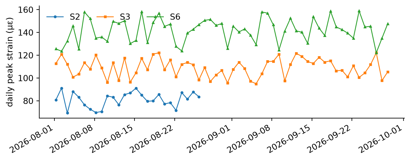
The division of labor is the point. The database filters, joins, and aggregates, which it does quickly and without loading anything it does not need. pandas takes over for the time-series work of Lecture 8 (resampling, rolling statistics, plotting). Once the result is pivoted, S2’s silence shows up as 33 missing days in its column, and Figure 11.2 shows what those numbers look like.
Figure 11.2: Daily peak strain of the three strain gauges, loaded with a single query. S2, on the Mill Creek Bridge, stops reporting after August 26.
11.9.4 Other Database Servers
sqlite3 reaches only SQLite. Every other system has its own Python driver, such as pymysql or mysql-connector-python for MySQL and psycopg for PostgreSQL, each with small differences in how it connects and which placeholder it expects. SQLAlchemy puts one interface over all of them. A connection is described by a URL, and pandas accepts a SQLAlchemy connection wherever it accepts a sqlite3 one:
from sqlalchemy import create_engine, textengine = create_engine("sqlite:///bridges.sqlite")with engine.connect() as conn: n = pd.read_sql_query(text("SELECT COUNT(*) AS n FROM Reading"), conn)print(n)
     n
0  321
Moving the same code to a MySQL server changes only the URL, to something like mysql+pymysql://user:password@host/monitoring (with the pymysql driver installed). PostgreSQL’s begins postgresql+psycopg://. The SQL itself moves as well as its dialect allows. Two habits make the move easier: write standard SQL where there is a choice, and keep passwords out of the code. SQLAlchemy can also build queries from Python objects and map tables to classes. Those tools are worth learning for a large application and unnecessary for this course.
11.10 Putting It All Together
The engineer’s question from the start of Lecture 9 can now be answered in one statement: which strain gauges on bridges built before 1950 have gone silent this month, and who inspected those bridges last? Each clause below comes from one section of this lecture.
SELECT s.sensor_id, b.name AS bridge, (SELECTMAX(r.time) FROM Reading AS rWHERE r.sensor_id = s.sensor_id) AS last_heard, -- correlated subquery e.name AS last_inspector, i.dateAS inspectedFROM Sensor AS sJOIN Bridge AS b ON b.bridge_id = s.bridge_id -- inner joinLEFTJOIN Inspects AS i -- outer join: keepON i.bridge_id = b.bridge_id -- uninspected bridgesAND i.date= (SELECTMAX(date) FROM InspectsWHERE bridge_id = b.bridge_id) -- latest inspectionLEFTJOIN Engineer AS e ON e.emp_id = i.emp_id -- chain of joinsWHERE s.type='strain_gauge'-- selectionAND b.year_built <1950ANDNOTEXISTS (SELECT*FROM Reading AS r -- "gone silent"WHERE r.sensor_id = s.sensor_idAND r.time>='2026-09-01');
Table 11.20: The answer to the engineer’s question.
sensor_id
bridge
last_heard
last_inspector
inspected
S2
Mill Creek Bridge
2026-08-26T06:00:00Z
Dana Kowalski
2026-05-20
Strain gauge S2 on the Mill Creek Bridge has been silent since August 26. It is the sensor the data-quality check in Lecture 9 had already flagged, and Dana Kowalski inspected its bridge last, on May 20. The question reached across five tables and needed a filter, two kinds of join, and three subqueries. No time series on its own could have answered it.
This lecture turned Lecture 9’s design into a working database:
DDL declared the schema, and its constraints made the database reject impossible data.
DML changed the instance, with transactions keeping related changes together.
SELECT answered questions about one table, and joins and subqueries answered questions that span several.
The algebra remained underneath all of it, the place where a query’s meaning can be checked.
Python tied the database to the programs that fill it and the analyses that read it.
Lecture 11 asks what makes one working schema better than another: why some designs invite update anomalies, how normalization removes them, what transactions guarantee, and what indexes cost. Assignment 2’s Tasks 4 and 5 put this lecture to work, on the database you design for the campus sensing kits.
11.11 Exercises
Defining a water network (LO1). Write CREATE TABLE statements for four relations of the water utility in Lecture 9’s active learning (Section 10.3.7): Junction(junction_id, elevation_m), Pipe(asset_no, diameter_mm, material, install_year, upstream_id, downstream_id), Logger(serial, junction_id), and Reading(serial, seq_no, time, pressure_kpa). Declare the keys and foreign keys, and add constraints that forbid a pipe of non-positive diameter and a pipe that runs from a junction to itself.
TipSolution
CREATETABLE Junction ( junction_id TEXT PRIMARYKEY, elevation_m REAL);CREATETABLE Pipe ( asset_no TEXT PRIMARYKEY, diameter_mm REALNOTNULLCHECK (diameter_mm >0), material TEXT, install_year INTEGER, upstream_id TEXT NOTNULLREFERENCES Junction (junction_id), downstream_id TEXT NOTNULLREFERENCES Junction (junction_id),CHECK (upstream_id <> downstream_id));CREATETABLE Logger ( serial TEXT PRIMARYKEY, junction_id TEXT NOTNULLREFERENCES Junction (junction_id));CREATETABLE Reading ( serial TEXT NOTNULLREFERENCES Logger (serial), seq_no INTEGERNOTNULL,time TEXT NOTNULL, pressure_kpa REAL,PRIMARYKEY (serial, seq_no));
The roles upstream and downstream become two foreign keys into the same table, named for their roles. The rule that they differ involves two columns, so it is written as a table-level CHECK. Reading’s composite key reflects its status as a weak entity set, numbered within its logger.
Keeping the database right (LO1). On the bridge database:
Record that engineer E1 inspected the Riverside Bridge on 2026-09-28 with a rating of 6.
The installation year of S3 was entered wrongly and should be 2020. Correct it.
The manufacturer Kestrel Gauges changes its name to Kestrel Systems. Explain why UPDATE Manufacturer SET mfr_name = 'Kestrel Systems' WHERE mfr_name = 'Kestrel Gauges'; fails, and give two ways to make the change.
UPDATE Sensor SET install_year = 2020 WHERE sensor_id = 'S3'; (and check that it reports one row changed).
Three sensors refer to Kestrel Gauges through their foreign key mfr_name. Renaming the key would leave them pointing at a manufacturer that no longer exists, so the foreign key rejects the update. One way is to do it in steps, in one transaction: insert Kestrel Systems, update the three sensors to point at it, then delete Kestrel Gauges. Another is to declare the foreign key with REFERENCES Manufacturer (mfr_name) ON UPDATE CASCADE, so that the database updates the referring rows itself. The episode also shows why many designers prefer a meaningless identifier (mfr_id) as a key: names change, and identifiers need not.
Summaries (LO2). Write queries for the following, and give their results.
The number of September readings from each sensor, most first. Why does S2 not appear, and which later section shows how to make it appear with a count of 0?
For each sensor type, the number of sensors and the earliest installation year.
The sensors whose peak value in the record exceeds their own mean by more than 15%.
TipSolution
SELECT sensor_id, COUNT(*) AS n FROM Reading WHERE time >= '2026-09-01' GROUP BY sensor_id ORDER BY n DESC; gives 28 for each of S1, S3, S4, S5, and S6. S2 has no September rows, so after WHERE there is nothing to form a group from. A group exists only if at least one row belongs to it. A LEFT JOIN from Sensor to Reading, with the date condition in ON and COUNT(r.seq_no), lists S2 with 0 (Section 11.6.2).
SELECT type, COUNT(*) AS n, MIN(install_year) AS first FROM Sensor GROUP BY type; gives accelerometer 2 and 2019, strain gauge 3 and 2019, temperature 1 and 2022.
SELECT sensor_id, MAX(value) AS peak, ROUND(AVG(value), 1) AS mean FROM Reading GROUP BY sensor_id HAVING MAX(value) > 1.15 * AVG(value); returns S1 (14.9 against 12.1), S4 (24.9 against 20.0), and S5 (25.7 against 21.8). The condition is about each group’s aggregates, so it belongs in HAVING.
Across tables (LO3, LO4). Write queries for the following.
Each manufacturer with the number of sensors it supplied, including manufacturers that supplied none.
The names of the engineers who have inspected a bridge that carries an accelerometer.
For each bridge, the time of its most recent reading from any sensor, including bridges that have no sensors.
TipSolution
SELECT m.mfr_name, COUNT(s.sensor_id) AS n FROM Manufacturer AS m LEFT JOIN Sensor AS s ON s.mfr_name = m.mfr_name GROUP BY m.mfr_name; gives Borealis Instruments 3, Kestrel Gauges 3, and Meridian Sensing 0. The zero depends on counting a column of the right table.
SELECT DISTINCT e.name FROM Engineer AS e JOIN Inspects AS i ON i.emp_id = e.emp_id WHERE i.bridge_id IN (SELECT bridge_id FROM Sensor WHERE type = 'accelerometer'); gives Ben Okafor, Chen Wei, and Dana Kowalski. The accelerometers are on B1 and B3, and those three engineers have inspected one of them. A join with Sensor in place of the subquery also works, and then DISTINCT is needed even more.
SELECT b.name, MAX(r.time) AS last_reading FROM Bridge AS b LEFT JOIN Sensor AS s ON s.bridge_id = b.bridge_id LEFT JOIN Reading AS r ON r.sensor_id = s.sensor_id GROUP BY b.bridge_id, b.name; gives 2026-09-28T06:00:00Z for the three instrumented bridges and NULL for the Station Street Bridge. The Mill Creek Bridge’s latest reading comes from S1: a bridge whose newest reading is recent can still have a silent sensor, which is why the engineer’s question is asked per sensor.
Algebra and SQL (LO5).
Translate \(\pi_{\text{name}}\big(\sigma_{\text{length\_m} > 200}(\text{Bridge}) \bowtie \sigma_{\text{type} = \text{'strain\_gauge'}}(\text{Sensor})\big)\) into SQL, and give the result.
Translate SELECT DISTINCT e.name FROM Engineer AS e, Inspects AS i WHERE e.emp_id = i.emp_id AND i.rating <= 5; into relational algebra, and give the result.
Lecture 9’s Exercise 5(b) asked for the bridges that have an accelerometer but no strain gauge. Write it in SQL with a set operator.
TipSolution
SELECT DISTINCT b.name FROM Bridge AS b JOIN Sensor AS s ON s.bridge_id = b.bridge_id WHERE b.length_m > 200 AND s.type = 'strain_gauge'; gives the Riverside Bridge and the Harbor Bridge. Moving both selections into WHERE is allowed because selections can be pushed through a join in either direction.
\(\pi_{\text{name}}\big(\sigma_{\text{rating} \le 5}(\text{Engineer} \bowtie \text{Inspects})\big)\). The natural join is safe here because the two relations share only emp_id. The result is Ana Ruiz, Chen Wei, and Dana Kowalski.
SELECT bridge_id FROM Sensor WHERE type = 'accelerometer' EXCEPT SELECT bridge_id FROM Sensor WHERE type = 'strain_gauge'; returns no rows, as in Lecture 9: both bridges with accelerometers also carry strain gauges.
A monitoring function (LO6). Write a Python function strain_summary(con, bridge_id) that returns a DataFrame with one row per strain gauge on the given bridge, holding the number of valid readings, their mean, and their peak. Why should bridge_id reach the query as a parameter rather than through an f-string?
TipSolution
import pandas as pddef strain_summary(con, bridge_id): query =""" SELECT r.sensor_id, COUNT(r.value) AS n_valid, ROUND(AVG(r.value), 1) AS mean, MAX(r.value) AS peak FROM Reading AS r JOIN Sensor AS s ON s.sensor_id = r.sensor_id WHERE s.bridge_id = ? AND s.type = 'strain_gauge' GROUP BY r.sensor_id """return pd.read_sql_query(query, con, params=(bridge_id,))con = sqlite3.connect("bridges.sqlite")print(strain_summary(con, "B3"))
  sensor_id  n_valid   mean   peak
0        S6       59  141.8  158.9
The database does the joining, filtering, and aggregation, and returns only one row per gauge. The parameter keeps the value out of the SQL text. A bridge ID typed by a user, or read from a file, can then never change what the statement does, and a value containing a quote cannot break it.
Codd, E. F. 1970. “A Relational Model of Data for Large Shared Data Banks.”Communications of the ACM 13 (6): 377–87. https://doi.org/10.1145/362384.362685.
Garcia-Molina, Hector, Jeffrey D. Ullman, and Jennifer Widom. 2009. Database Systems: The Complete Book. 2nd ed. Pearson Prentice Hall.