By the end of this lecture, students should be able to:
Identify insertion, update, and deletion anomalies in a poorly designed schema
Derive functional dependencies from the properties of the data, and compute closures and keys of relations
Normalize a schema through the normal forms, decomposing a relation up to Boyce-Codd Normal Form (BCNF) when possible
Explain what transactions and the ACID properties guarantee, and why they matter for concurrent data collection
Describe how indexes speed up queries and what they cost, and weigh normalization against denormalization for high-volume time-series workloads
NoteTopics Covered
Redundancy and the update, deletion, and insertion anomalies
Functional dependencies, Armstrong’s axioms, closures, and keys
First, second, and third normal forms, and Boyce-Codd Normal Form
The BCNF decomposition algorithm, lossless joins, and dependency preservation
Optional: multivalued dependencies and Fourth Normal Form
Transactions, the ACID properties, isolation levels, and concurrency in SQLite
B-tree indexes, query plans, and what indexes cost
Normalization versus denormalization for time-series data
12.1.1 Before You Begin
This lecture asks what makes one working schema better than another, so it builds on the two before it: Lecture 9’s bridge-monitoring program and the nine relations it was translated into (Section 10.7.5), and Lecture 10’s SQL, including its brief first look at transactions (Section 11.4.2). The examples run on the same database, bridges.sqlite, a copy of Lecture 10’s file, built by Lecture 10’s script make_bridges_db.py; the city and everything in it are hypothetical.
The index experiments in Section 12.6 need more rows than a few bridges produce. They use ten synthetic sensors reporting once a minute for the 30 days of September 2026, 432,000 rows in all, which the script make_minute_readings.py generates (python make_minute_readings.py writes minute_readings.sqlite). Only Python’s standard library is needed.
12.2 Why Design Matters
Lecture 9 turned an E/R diagram into nine relations, and Lecture 10 built them in SQLite and queried them. Nothing forced that particular set of tables. The same facts could live in three tables, in nine, or in one big table exported from a spreadsheet, and SQL would accept every one of those designs and answer queries on it. The designs differ in what they let go wrong: some let the database contradict itself, lose facts nobody meant to delete, or refuse facts it should accept. This section shows those failures on real rows. The rest of the lecture develops the theory that predicts them and removes them, following Chapter 3 of Garcia-Molina, Ullman, and Widom (Garcia-Molina et al. 2009).
12.2.1 One Big Table
Suppose that instead of three tables for sensors, bridges, and manufacturers, the city had kept a single sheet with one row per sensor and everything known about it. That sheet is not hypothetical: it is exactly what the join of Lecture 10 produces, and what many monitoring programs keep in practice.
SELECT s.sensor_id, s.type, s.install_year, b.bridge_id, b.name AS bridge_name, b.year_built, b.length_m, m.mfr_name, m.countryFROM Sensor AS sJOIN Bridge AS b ON b.bridge_id = s.bridge_idJOIN Manufacturer AS m ON m.mfr_name = s.mfr_name;
Table 12.1: Inventory: one row per sensor, with its bridge and manufacturer.
sensor_id
type
install_year
bridge_id
bridge_name
year_built
length_m
mfr_name
country
S1
accelerometer
2019
B1
Mill Creek Bridge
1931
118
Kestrel Gauges
USA
S2
strain_gauge
2019
B1
Mill Creek Bridge
1931
118
Kestrel Gauges
USA
S3
strain_gauge
2021
B2
Riverside Bridge
1959
240
Borealis Instruments
Canada
S4
accelerometer
2021
B3
Harbor Bridge
1972
610
Borealis Instruments
Canada
S5
temperature
2022
B3
Harbor Bridge
1972
610
Kestrel Gauges
USA
S6
strain_gauge
2022
B3
Harbor Bridge
1972
610
Borealis Instruments
Canada
Call this relation Inventory. It is convenient: every question about a sensor is answered from one row, with no join. It is also redundant. The Harbor Bridge’s name, year, and length are stored three times, once for each of its sensors, and “Kestrel Gauges, USA” and “Borealis Instruments, Canada” three times each. Redundancy wastes some space, but space is cheap. The real cost is that every repeated fact is a fact that can be stored inconsistently.
12.2.2 Three Anomalies
Redundancy turns into three kinds of failure, called anomalies, each triggered by one of the three ways of changing data (Garcia-Molina et al. 2009, sec. 3.3.1). To see them happen, the next queries run on a copy of Table 12.1 stored as a table named Inventory.
An update anomaly occurs when a fact stored in several rows is changed in only some of them. A new survey puts the Harbor Bridge at 612 m, and the person making the change finds the first matching row:
UPDATE Inventory SET length_m =612WHERE sensor_id ='S4';SELECT bridge_name, COUNT(DISTINCT length_m) AS lengths_on_recordFROM InventoryGROUPBY bridge_name;
Table 12.2: After a one-row update, the Harbor Bridge has two lengths.
bridge_name
lengths_on_record
Harbor Bridge
2
Mill Creek Bridge
1
Riverside Bridge
1
Nothing rejected the update, and now the database holds two lengths for one bridge. Which is right can no longer be decided from the data.
A deletion anomaly occurs when deleting one fact deletes another that nobody meant to remove. The two sensors on the Mill Creek Bridge are retired:
DELETEFROM Inventory WHERE sensor_id IN ('S1', 'S2');SELECTDISTINCT bridge_name FROM Inventory;
Table 12.3: After the Mill Creek sensors are removed, so is the Mill Creek Bridge.
bridge_name
Riverside Bridge
Harbor Bridge
The bridge still stands, but the database no longer knows it exists, when it was built, or how long it is.
An insertion anomaly occurs when a fact cannot be recorded without another, unrelated fact. Table 12.1 already shows one. The city owns four bridges and has approved three manufacturers, but the Station Street Bridge and Meridian Sensing appear nowhere in it, because neither is attached to a sensor. Inventory has room for a bridge only in a sensor’s row. To record a new bridge before instrumenting it, someone would have to invent a sensor or leave its sensor_id null, and sensor_id identifies the row.
CautionConcept Check: Name the anomaly
Using Inventory (Table 12.1), classify each problem as an update, deletion, or insertion anomaly: (a) Borealis Instruments relocates to the United States; (b) the city wants to record its purchase contract with Meridian Sensing before any sensor arrives; (c) S3, the only sensor on the Riverside Bridge, fails and is removed.
TipAnswer
Update anomaly: the country is stored in three rows, and changing only some of them leaves Borealis in two countries. (b) Insertion anomaly: a manufacturer can appear only in a sensor’s row. (c) Deletion anomaly: removing S3’s row removes the only record of the Riverside Bridge.
12.2.3 Splitting the Table
All three anomalies have one cause: Inventory mixes facts about three different things, and a fact about a bridge is repeated once per sensor. Lecture 9’s schema keeps them apart. Bridge holds one row per bridge, Manufacturer one row per manufacturer, and Sensor one row per sensor, with foreign keys to the other two. Each fact is stored once, so it can be changed in one place; a bridge has a row of its own, so it neither needs a sensor to exist nor disappears with one. Lecture 9 stated the principle as “say everything once” (Section 10.3.7), and the join that built Table 12.1 shows that nothing was lost by following it: Inventory can always be recomputed from the three tables.
That decomposition was found by judgment, from an E/R diagram. Judgment does not scale, and it gives no way to tell whether a design is finished or why it is safe to split a table one way and not another. The next two sections replace it with a procedure. Functional dependencies record which facts determine which (Section 12.3), and normal forms say which dependencies a well-designed relation may contain, with an algorithm that splits a relation until it complies (Section 12.4).
12.3 Functional Dependencies
To decide mechanically that Inventory repeats bridge facts, a design method needs to know something the rows alone cannot tell it: that a bridge’s ID pins down its name, year, and length. That is a statement about the world the data describes, not about any one instance, and a functional dependency is the notation for writing it down.
12.3.1 What a Functional Dependency Says
A functional dependency (FD) on a relation \(R\) is a statement
\[X \rightarrow Y,\]
read “\(X\) functionally determines \(Y\)”, where \(X\) and \(Y\) are sets of attributes of \(R\). It says that any two tuples of \(R\) that agree on all the attributes of \(X\) must also agree on all the attributes of \(Y\)(Garcia-Molina et al. 2009, sec. 3.1.1). The name comes from functions: an FD says that \(Y\) is a function of \(X\), so that knowing the \(X\)-values of a tuple leaves only one possibility for its \(Y\)-values. Sets of attributes are written without braces when that is unambiguous, so \(\text{bridge\_id} \rightarrow \text{bridge\_name}, \text{year\_built}\) means \(\{\text{bridge\_id}\} \rightarrow \{\text{bridge\_name}, \text{year\_built}\}\).
A key, in this vocabulary, is a set of attributes that functionally determines every attribute of the relation, and is minimal: no proper subset determines everything too (Garcia-Molina et al. 2009, sec. 3.1.3). A set that determines everything but may not be minimal is a superkey. These are the keys of Lecture 9 (Section 10.5.3), restated so that they can be computed.
12.3.2 Finding the Dependencies of a Relation
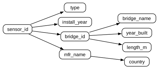
FDs come from the rules of the program that produces the data, not from inspecting a table. For Inventory, the city’s rules give three:
\(F_1\) holds because the city issues each bridge an ID, and a bridge has one name, one year of construction, and one length. \(F_2\) holds because a sensor has one type and one installation year, is on one bridge (the many-one Monitors relationship of Lecture 9), and has one manufacturer. \(F_3\) assumes that each manufacturer is based in one country. Figure 12.1 draws them.
Figure 12.1: The functional dependencies of Inventory. An arrow from one attribute to another means the first determines the second.
An instance can refute an FD but never prove one. Lecture 9’s concept check made the same point about keys (Section 10.5.4). In Table 12.1, no two rows share a year_built with different bridge names, so the instance happens to satisfy \(\text{year\_built} \rightarrow \text{bridge\_name}\). It is still not a dependency, because nothing stops the city from acquiring a second bridge built in 1972. Data can, however, find violations of an FD you believe in. Grouping by the left side and counting distinct right-side values finds every group that breaks the rule, which is a useful check on a spreadsheet before it is loaded into a database:
-- groups that violate bridge_id -> length_mSELECT bridge_id, COUNT(DISTINCT length_m) AS n_valuesFROM InventoryGROUPBY bridge_idHAVINGCOUNT(DISTINCT length_m) >1;
Table 12.4: The check finds the inconsistent length left by the update of Table 12.2.
bridge_id
n_values
B3
2
TipActive Learning: Rules or coincidences?
Work in pairs, eight minutes. A building-energy dashboard exports this table, MeterLog:
meter_id
building
floor_area_m2
utility_account
time
kwh
M1
North Lab
12500
A-1001
2026-09-14T00:00Z
41.2
M1
North Lab
12500
A-1001
2026-09-14T01:00Z
39.8
M2
Civil Annex
9800
A-1001
2026-09-14T00:00Z
27.5
M2
Civil Annex
9800
A-1001
2026-09-14T01:00Z
26.9
M3
Library
31000
A-2040
2026-09-14T00:00Z
88.1
Each meter measures one building, and each building has one floor area and is billed to one utility account (an account may cover several buildings). Write down the FDs these rules imply. Then find one FD that the instance satisfies but the rules do not guarantee.
NoteWhat to look for
The rules give \(\text{meter\_id} \rightarrow \text{building}\), \(\text{building} \rightarrow \text{floor\_area\_m2}, \text{utility\_account}\), and, because a meter reports one value per hour, \(\text{meter\_id}, \text{time} \rightarrow \text{kwh}\). Coincidences include \(\text{floor\_area\_m2} \rightarrow \text{building}\) (the three areas happen to differ) and \(\text{kwh} \rightarrow \text{meter\_id}\) (no two readings happen to be equal). The reverse of a real rule is a common trap: \(\text{utility\_account} \rightarrow \text{building}\) is refuted by account A-1001, which covers two buildings.
12.3.3 Reasoning with Dependencies
The three FDs of Inventory imply others. Since a sensor determines its bridge, and a bridge determines its length, a sensor determines the length of the bridge it is on, \(\text{sensor\_id} \rightarrow \text{length\_m}\), even though nobody wrote that down. A design method has to see such consequences, because they are exactly where hidden redundancy lives. A few rules generate all of them (Garcia-Molina et al. 2009, sec. 3.2).
An FD \(X \rightarrow Y\) is trivial if \(Y \subseteq X\), such as \(\text{bridge\_id}, \text{bridge\_name} \rightarrow \text{bridge\_id}\). Trivial FDs hold in every relation and say nothing about the data. The right side of an FD can be split and combined freely: \(X \rightarrow A, B\) holds exactly when both \(X \rightarrow A\) and \(X \rightarrow B\) hold. The left side cannot. \(\text{meter\_id}, \text{time} \rightarrow \text{kwh}\) is true of MeterLog, while neither \(\text{meter\_id} \rightarrow \text{kwh}\) nor \(\text{time} \rightarrow \text{kwh}\) is.
Three rules, known as Armstrong’s axioms, derive every FD that follows from a given set:
Reflexivity. If \(Y \subseteq X\), then \(X \rightarrow Y\). (Trivial FDs hold.)
Augmentation. If \(X \rightarrow Y\), then \(XZ \rightarrow YZ\) for any set of attributes \(Z\), where \(XZ\) is shorthand for \(X \cup Z\).
Transitivity. If \(X \rightarrow Y\) and \(Y \rightarrow Z\), then \(X \rightarrow Z\).
The rules are sound, meaning that everything they derive does follow from the given FDs, and complete, meaning that everything that follows can be derived with them. Transitivity alone gives \(\text{sensor\_id} \rightarrow \text{length\_m}\) from \(F_2\) and \(F_1\) (after splitting their right sides). Deriving FDs by hand, one axiom at a time, is slow and easy to get wrong, though. The next subsection gives a procedure that answers the practical question directly.
12.3.4 Closures
Every design question in this lecture reduces to one: given these attributes, what else do they determine? Is sensor_id a key? Does bridge_id determine mfr_name? Both are answered by the closure. The closure of a set of attributes \(X\) under a set of FDs \(F\), written \(X^+\), is the set of all attributes \(A\) such that \(X \rightarrow A\) follows from \(F\)(Garcia-Molina et al. 2009, sec. 3.2.4). It is computed by a simple fixed-point loop:
Start with \(X^+ = X\).
Look for an FD \(L \rightarrow R\) in \(F\) whose whole left side is already in \(X^+\), and whose right side is not. Add \(R\) to \(X^+\).
Repeat step 2 until no FD adds anything. Then \(X^+\) is complete.
Each step uses only transitivity and the splitting rule, which is why the result is correct. The loop ends because each step adds at least one attribute, and there are finitely many.
Here is the loop for \(\{\text{sensor\_id}\}^+\), with the FDs checked in the order \(F_1, F_2, F_3\):
No FD adds anything more, so the closure has 9 attributes.
\(F_1\) could not fire on the first pass, because bridge_id was not yet in the closure. It fired on the second pass, once \(F_2\) had put bridge_id there. That chain, \(\text{sensor\_id} \rightarrow \text{bridge\_id} \rightarrow \text{bridge\_name}\), is the transitivity that put the Harbor Bridge’s name into three rows. By contrast, \(\{\text{bridge\_id}\}^+ = \{\text{bridge\_id}, \text{bridge\_name}, \text{year\_built}, \text{length\_m}\}\): after \(F_1\) fires, neither \(F_2\) nor \(F_3\) has its left side in the closure.
The closure also tests whether an FD follows from others: \(X \rightarrow Y\) follows from \(F\) exactly when \(Y \subseteq X^+\). So \(\text{sensor\_id} \rightarrow \text{country}\) follows, because country is in \(\{\text{sensor\_id}\}^+\). And \(\text{bridge\_id} \rightarrow \text{mfr\_name}\) does not, because a bridge can carry sensors from several manufacturers.
NoteThe closure algorithm in Python
The loop is short enough to write out. Each FD is a pair of sets of attribute names.
def closure(attrs, fds): result =set(attrs) changed =Truewhile changed: changed =Falsefor lhs, rhs in fds:if lhs <= result andnot rhs <= result: # new attributes result |= rhs changed =Truereturn resultinventory_fds = [ ({"bridge_id"}, {"bridge_name", "year_built", "length_m"}), ({"sensor_id"}, {"type", "install_year", "bridge_id", "mfr_name"}), ({"mfr_name"}, {"country"}),]sorted(closure({"bridge_id"}, inventory_fds))
A set of attributes \(X\) is a superkey of \(R\) exactly when \(X^+\) contains every attribute of \(R\). It is a key when, in addition, no proper subset of \(X\) is a superkey (Garcia-Molina et al. 2009, sec. 3.2.4). For Inventory, \(\{\text{sensor\_id}\}^+\) is all nine attributes, so sensor_id is a superkey; a single attribute has no proper nonempty subsets, so it is a key. \(\{\text{sensor\_id}, \text{bridge\_id}\}\) is a superkey too, but not a key, because it contains sensor_id.
Finding all the keys could mean testing every subset of attributes, \(2^9 = 512\) of them for Inventory. One observation cuts the work sharply. An attribute that appears on the right side of no FD can only be in a closure if it was there from the start, so it belongs to every key. sensor_id is on no right side in Figure 12.1, so every key of Inventory contains it. Since sensor_id is already a key on its own, it is the only key: any other superkey contains it and is therefore not minimal. In general, start from the attributes on no right side, compute their closure, and add attributes one at a time only if that closure falls short.
TipTry it: closures and keys
Tick a set of attributes of Inventory to compute its closure under \(F_1\), \(F_2\), and \(F_3\). The steps show which FD added what, and the verdict says whether the set is a superkey, a key, or neither. Try bridge_id and mfr_name together, then add type, then swap in sensor_id.
closureReport = {const {result, steps} =closureSteps(pickedAttrs, invFDs);const all = invAttrs.every(a => result.has(a));const superSub = pickedAttrs.some(x => invAttrs.every(a =>closureSteps(pickedAttrs.filter(y => y !== x), invFDs).result.has(a)));const verdict = pickedAttrs.length===0?"Pick at least one attribute.":!all ?"Not a superkey: the closure misses "+ invAttrs.filter(a =>!result.has(a)).join(", ") +".": superSub ?"A superkey, but not a key: an attribute can be removed and the rest still determines everything.":"A key: the closure is every attribute, and removing any picked attribute breaks that.";returnhtml`<div class="sql-out"> <p><strong>Closure:</strong> {${invAttrs.filter(a => result.has(a)).join(", ")}}</p> <ol>${steps.map(s =>html`<li>${s.fd} applies: add ${s.added.join(", ")}</li>`)}</ol> <p><strong>Verdict:</strong> ${verdict}</p></div>`;}
CautionConcept Check: The key of an inspection record
Suppose Lecture 9’s Inspects relation also carried each bridge’s name: Inspects(emp_id, bridge_id, bridge_name, date, rating), with the FDs \(\text{emp\_id}, \text{bridge\_id} \rightarrow \text{date}, \text{rating}\) and \(\text{bridge\_id} \rightarrow \text{bridge\_name}\). What is \(\{\text{bridge\_id}\}^+\)? What are the keys?
TipAnswer
\(\{\text{bridge\_id}\}^+ = \{\text{bridge\_id}, \text{bridge\_name}\}\), so bridge_id alone is not a superkey. emp_id and bridge_id appear on no right side, so both are in every key. Their closure is all five attributes, so \(\{\text{emp\_id}, \text{bridge\_id}\}\) is a superkey, and it is the only key.
12.4 Normal Forms and Decomposition
We now know the FDs of Inventory and its key, but not yet what is wrong with them. The problem is visible in Figure 12.1: bridge_id and mfr_name determine other attributes without being keys. Each distinct bridge_id may appear in many rows, and every such row repeats what \(F_1\) says about it. A normal form is a condition on a relation’s FDs that rules out such patterns. The normal forms were introduced one at a time, as each was found to leave some anomaly in place, and they form a ladder: every relation in Boyce-Codd Normal Form is in third normal form, every relation in third normal form is in second, and every relation in second is in first (Codd 1972; Garcia-Molina et al. 2009, sec. 3.3 and 3.5). This section climbs the ladder and ends with an algorithm that takes any relation to the top.
One more term is needed. An attribute is prime if it belongs to at least one key, and nonprime otherwise. In Inventory, sensor_id is prime and the other eight attributes are nonprime.
12.4.1 First Normal Form
A relation is in first normal form (1NF) if every value is atomic: a single number, string, or date, never a list or a set. The relational model of Lecture 9 builds this in (Section 10.3.2), so every relation in this course is in 1NF by construction. Spreadsheets are not. A column sensors holding “S4, S5, S6” in the Harbor Bridge’s row cannot be joined, counted, or constrained by a foreign key, and a query for “bridges with sensor S5” must pick strings apart. The cure is to store one value per row: here, one row per sensor with a bridge_id pointing back, which is Sensor.
12.4.2 Second and Third Normal Forms
A relation is in second normal form (2NF) if no nonprime attribute depends on part of a key, that is, on a proper subset of a key. The augmented Inspects of the last concept check is not in 2NF. Its key is \(\{\text{emp\_id}, \text{bridge\_id}\}\), and the nonprime bridge_name depends on bridge_id alone. The name of a bridge is repeated in every inspection of that bridge, with the three anomalies to match. A relation whose keys are all single attributes has no proper parts of keys to depend on, so it is automatically in 2NF. Inventory is in 2NF, and still full of anomalies, so 2NF is not enough.
A relation is in third normal form (3NF) if, for every nontrivial FD \(X \rightarrow A\) that holds in it (with \(A\) a single attribute), \(X\) is a superkey or\(A\) is prime (Garcia-Molina et al. 2009, sec. 3.5.1). Inventory fails: in \(\text{bridge\_id} \rightarrow \text{bridge\_name}\), bridge_id is not a superkey and bridge_name is not prime. Many texts phrase 3NF as “no nonprime attribute depends on a key transitively, through another nonprime attribute”, which is the pattern \(\text{sensor\_id} \rightarrow \text{bridge\_id} \rightarrow \text{bridge\_name}\) exactly. The definition above is the precise one, and it also covers relations with several keys.
12.4.3 Boyce-Codd Normal Form
3NF’s escape clause, “or \(A\) is prime”, lets some redundancy through (Section 12.4.6 shows a case). Drop it and the result is the simplest and strongest of the four definitions. A relation \(R\) is in Boyce-Codd Normal Form (BCNF) if, for every nontrivial FD \(X \rightarrow Y\) that holds in \(R\), \(X\) is a superkey of \(R\)(Garcia-Molina et al. 2009, sec. 3.3.3). In words: the only things that determine other things are keys.
Why this removes the anomalies is worth one sentence. If \(X\) is a superkey, no two rows share an \(X\)-value, so whatever \(X\) determines is stated once, in one row, and cannot be repeated or contradicted. Every FD of Inventory other than \(F_2\) violates BCNF, because neither bridge_id nor mfr_name is a superkey. The three tables of Lecture 9 are each in BCNF: in Bridge the only nontrivial FDs have bridge_id on the left, and it is Bridge’s key, and likewise for Sensor and Manufacturer.
Table 12.5: The four normal forms, from weakest to strongest, and where Inventory stands.
Normal form
Forbids
Inventory
1NF
non-atomic values (lists, sets)
satisfies
2NF
a nonprime attribute depending on part of a key
satisfies (its key is one attribute)
3NF
\(X \rightarrow A\) with \(X\) not a superkey and \(A\) nonprime
violates (\(F_1\), \(F_3\))
BCNF
\(X \rightarrow A\) with \(X\) not a superkey
violates (\(F_1\), \(F_3\))
CautionConcept Check: One-attribute keys
A colleague argues that any table whose key is a single ID column, such as sensor_id or meter_id, is automatically well designed. Which normal form does a single-attribute key guarantee, and which does it not?
TipAnswer
It guarantees 2NF, since a one-attribute key has no proper parts for anything to depend on. It does not guarantee 3NF or BCNF: Inventory’s key is the single attribute sensor_id, yet bridge_id and mfr_name determine other attributes without being keys, which is where its anomalies come from. Adding an ID column to a spreadsheet does not normalize it.
12.4.4 Decomposing into BCNF
Knowing that Inventory violates BCNF is only half the job; the design method must also say how to fix it. The fix is to split the relation along a violating FD, and repeat (Garcia-Molina et al. 2009, sec. 3.3.4):
If \(R\) is in BCNF, stop.
Otherwise, pick a violating FD \(X \rightarrow Y\) and compute \(X^+\).
Replace \(R\) by two relations: \(R_1 = X^+\), holding \(X\) and everything it determines, and \(R_2 = X \cup (R - X^+)\), holding \(X\) and everything else.
Work out which FDs hold in \(R_1\) and in \(R_2\), and apply the algorithm to each.
Splitting on \(X^+\) rather than on \(X \rightarrow Y\) alone moves everything \(X\) determines in one step. Keeping \(X\) in both halves is what lets the two be joined back together, as Section 12.4.5 shows.
On Inventory, take \(F_1\) first. \(\{\text{bridge\_id}\}^+ = \{\text{bridge\_id}, \text{bridge\_name}, \text{year\_built}, \text{length\_m}\}\), so \(R_1\) is those four attributes, and \(R_2\) keeps bridge_id with the other five attributes. \(R_1\) is in BCNF, since its only nontrivial FDs have bridge_id, its key, on the left. \(R_2\) still contains \(F_2\) and \(F_3\), and \(F_3\) violates BCNF there, since mfr_name does not determine sensor_id. Splitting \(R_2\) on \(\{\text{mfr\_name}\}^+ = \{\text{mfr\_name}, \text{country}\}\) gives two relations in BCNF. Figure 12.2 shows the result: Lecture 9’s Bridge, Manufacturer, and Sensor, recovered from the FDs alone.
Figure 12.2: BCNF decomposition of Inventory. Each split is on a violating FD; the leaves are in BCNF and are Lecture 9’s Bridge, Manufacturer, and Sensor relations.
Two remarks keep the algorithm honest. First, step 4 hides real work in general. The FDs of a piece are not just the given FDs that fit inside it, but everything that follows from \(F\) and fits inside it; with only three simple FDs this is easy to see, but in general it takes closures of subsets of the piece. Second, when a relation has several violations, the order in which they are chosen can change the final schema. Every result is in BCNF, but some fit the application better than others. For Inventory both orders give the same three tables.
12.4.5 Getting the Data Back: Lossless Joins
Splitting a table is safe only if the pieces can be put back together. The natural join of the pieces always contains every original row, so nothing can go missing. The danger is the opposite: the join can produce rows that were never there. Consider an arbitrary split of Sensor into (sensor_id, type, install_year, mfr_name) and (mfr_name, bridge_id), sharing mfr_name:
SELECT a.sensor_id, b.bridge_idFROM SensorMfr AS a JOIN MfrBridge AS b ON b.mfr_name = a.mfr_nameORDERBY a.sensor_id, b.bridge_id;
Table 12.6: Joining a bad split of Sensor back together: twelve rows where there were six.
sensor_id
bridge_id
S1
B1
S1
B3
S2
B1
S2
B3
S3
B2
S3
B3
S4
B2
S4
B3
S5
B1
S5
B3
S6
B2
S6
B3
Six of the twelve rows are false. S1, for one, appears on the Harbor Bridge, because both S1 and a Harbor Bridge sensor come from Kestrel Gauges. The decomposition has lost information by adding rows: the real pairing of sensors and bridges can no longer be told apart from the spurious one. Such a decomposition is called lossy; one whose join always returns exactly the original relation is lossless.
For a split into two relations there is a simple test. The decomposition of \(R\) into \(R_1\) and \(R_2\) is lossless exactly when the shared attributes \(R_1 \cap R_2\) functionally determine all of \(R_1\) or all of \(R_2\)(Garcia-Molina et al. 2009, sec. 3.4). The bad split fails: mfr_name determines neither sensor_id nor bridge_id. Every split made by the BCNF algorithm passes, by construction. The shared attributes are \(X\), and \(X^+ = R_1\), so each row of \(R_2\) matches exactly one row of \(R_1\). This is why the algorithm splits on \(X^+\) and keeps \(X\) in both halves. For decompositions into more than two pieces, Garcia-Molina et al. give a general test, the chase.
12.4.6 When BCNF Costs a Constraint
A decomposition can be lossless and still lose something else: the ability to enforce an FD by a key. Usually BCNF costs nothing of the kind, but there is one characteristic situation, overlapping keys, where it does. Consider how the city assigns inspectors. Suppose it runs three types of inspection (routine, underwater, and fracture-critical) and adopts two policies: each inspector is qualified for exactly one inspection type, and each bridge has exactly one assigned inspector for each type of inspection it needs. Assignment(bridge_id, insp_type, emp_id) records who inspects what:
bridge_id is on no right side, so it is in every key. Its closure is just itself, and the closures of its two pairs are \(\{\text{bridge\_id}, \text{insp\_type}\}^+ = \{\text{bridge\_id}, \text{insp\_type}, \text{emp\_id}\}\) and \(\{\text{bridge\_id}, \text{emp\_id}\}^+ = \{\text{bridge\_id}, \text{emp\_id}, \text{insp\_type}\}\). So Assignment has two keys, and they overlap in bridge_id. Every attribute is prime, so Assignment is in 3NF. It is not in BCNF, because emp_id determines insp_type without being a superkey. The violation shows up as redundancy in Table 12.7: that E2 does underwater inspections is stated twice, and that E3 does routine ones is stated twice.
The BCNF algorithm splits on \(\text{emp\_id} \rightarrow \text{insp\_type}\) into Qualification(emp_id, insp_type), with key emp_id, and Duty(bridge_id, emp_id), with key \(\{\text{bridge\_id}, \text{emp\_id}\}\). Both are in BCNF, and the split is lossless. But the second policy, \(\text{bridge\_id}, \text{insp\_type} \rightarrow \text{emp\_id}\), mentions attributes that no longer sit together in any table, so no key can enforce it. Assigning E3, a routine inspector, to the Mill Creek Bridge, which already has E4 for routine inspections, satisfies both tables’ keys:
INSERTINTO Duty VALUES ('B1', 'E3'); -- accepted: (B1, E3) is a new keySELECT d.bridge_id, q.insp_type, COUNT(*) AS inspectorsFROM Duty AS d JOIN Qualification AS q ON q.emp_id = d.emp_idGROUPBY d.bridge_id, q.insp_typeHAVINGCOUNT(*) >1;
Table 12.8: After the insert, the Mill Creek Bridge has two routine inspectors.
bridge_id
insp_type
inspectors
B1
routine
2
The two options are a genuine trade-off. BCNF removes the redundancy, but it gives up an FD that the database used to enforce for free with a primary key. Enforcing it again takes a check across tables, in a trigger or in the application. 3NF keeps Assignment whole, and with it the enforceable FD, at the price of repeating each inspector’s qualification. A classic result makes 3NF the safe fallback: every relation has a decomposition into 3NF that is both lossless and dependency-preserving, meaning every FD can still be checked within a single table (Bernstein 1976; Garcia-Molina et al. 2009, sec. 3.5). BCNF cannot always promise both. In practice most schemas reach BCNF with nothing lost, as Inventory did. When they do not, the choice depends on which is worse for the application: occasional redundancy, or a constraint that has to be enforced by code.
NoteOptional: Beyond BCNF
This material is not required. It shows that BCNF does not remove every kind of redundancy, and explains a design mistake that is common when one table records several independent lists.
Suppose the city records, for each bridge, the materials it is built of and the engineers who may inspect it, in one table BridgeFacts(bridge_id, material, emp_id). A bridge of steel and concrete with two eligible engineers needs four rows, one for every combination:
bridge_id
material
emp_id
B1
steel
E2
B1
steel
E4
B1
concrete
E2
B1
concrete
E4
No nontrivial FD holds: a bridge determines neither one material nor one engineer. The only key is all three attributes, so the table is in BCNF. Yet it is plainly redundant, and adding a third engineer means adding two rows, one per material. Forget one and the table claims that the new engineer may inspect the steel but not the concrete.
The dependency at work is a multivalued dependency (MVD), written \(\text{bridge\_id} \twoheadrightarrow \text{material}\). It says that the set of materials of a bridge is independent of everything else in the row, so every material must be paired with every engineer. Fourth normal form (4NF) is BCNF with MVDs in place of FDs, and its decomposition algorithm splits BridgeFacts into BridgeMaterial(bridge_id, material) and Eligible(bridge_id, emp_id) (Garcia-Molina et al. 2009, sec. 3.6). Normal forms beyond 4NF exist, such as fifth normal form, which handles dependencies among three or more tables, but they rarely matter in practice (Kent 1983). The signal to watch for is a table that combines two independent lists about the same thing.
12.5 Transactions and ACID
A well-designed schema says what the data should look like. It says nothing about what happens while the data is being changed, and in a sensing system the data is changing all the time. Readings arrive from many gateways at once, an importer may crash halfway through a batch, and a dashboard reads while the loggers write. Lecture 10 introduced the transaction as a way to make two deletions succeed or fail together (Section 11.4.2). This section asks what a database actually promises about transactions, and what happens when two programs write at the same time.
12.5.1 Two Writers, One Database
Suppose the city adds a small table, SensorSummary(sensor_id, n_readings), holding the number of readings received from each sensor, so that a dashboard can show the counts without scanning Reading. Two gateways, A and B, forward readings from strain gauge S3. Each one inserts its batch into Reading and then updates the count by the obvious method: read the old value, add the batch size, write the new value. S3 has 59 readings. A delivers 10 more, and B delivers 5 at almost the same moment:
Table 12.9: A lost update: each gateway’s write is correct on its own, but B overwrites A’s.
Step
Gateway A
Gateway B
n_readings stored
1
read n_readings: 59
59
2
read n_readings: 59
59
3
insert 10 readings; write 59 + 10 = 69
69
4
insert 5 readings; write 59 + 5 = 64
64
Reading now holds 74 rows for S3, but the summary says 64. Nothing failed, and each gateway did the right thing. The interleaving did the damage: B computed its new value from a count that A was about to change. This is a lost update, and it stays silent until someone notices that the dashboard disagrees with the data. A crash causes a similar problem. If A’s process dies after inserting its readings but before updating the count, the two tables disagree again.
12.5.2 The ACID Properties
A transaction is a sequence of reads and writes that the database treats as one unit. The guarantees a database makes about transactions are summarized by four properties, whose initials Haerder and Reuter arranged into the acronym ACID (Haerder and Reuter 1983; Garcia-Molina et al. 2009, sec. 6.6):
Atomicity. A transaction happens completely or not at all. If gateway A inserts its readings and updates the count inside one transaction, a crash between the two leaves neither in place: on restart, the database undoes the partial work. ROLLBACK, or a failed statement inside Python’s with con: block (Section 11.9.2), undoes it deliberately.
Consistency. A transaction that starts in a state satisfying the database’s rules also ends in one. The database checks the rules it has been told about (keys, foreign keys, CHECK constraints) and rejects a transaction that breaks them. Rules it has not been told about, such as “n_readings equals the number of rows in Reading”, are the application’s to keep, and atomicity and isolation are what make that possible.
Isolation. Concurrent transactions do not see each other’s intermediate states. At the strongest level, the result is as if the transactions had run one at a time, in some order. This property is called serializability, and it would have prevented Table 12.9: run one after the other, in either order, the gateways leave the count at 74.
Durability. Once COMMIT returns, the change survives a crash or a power failure. The database achieves this by waiting until the change is safely written to storage before it reports success, which, as Section 12.5.4 explains, is also why committing is slow.
For a monitoring program, atomicity and durability decide whether a crash loses or corrupts data. Isolation decides whether many writers and readers can share one database safely.
12.5.3 Isolation Levels
Serializability is expensive, because it can require one transaction to wait for another or be aborted and retried. The SQL standard therefore lets a transaction ask for weaker isolation, in exchange for exposure to named anomalies. Here they are, as they would appear to a report that counts S3’s readings while gateway A is loading a batch:
Dirty read: the report sees A’s uncommitted rows, then A rolls back. The report has counted readings that never existed.
Non-repeatable read: the report reads S3’s n_readings twice within its own transaction and gets 59, then 69, because A committed in between.
Phantom: the report runs SELECT COUNT(*) FROM Reading WHERE sensor_id = 'S3' twice and gets different answers, because new rows matching the condition appeared.
The standard defines four isolation levels by which of these they allow:
A transaction chooses its level with SET TRANSACTION ISOLATION LEVEL …. The defaults differ: PostgreSQL uses READ COMMITTED(The PostgreSQL Global Development Group 2026), and MySQL’s InnoDB engine uses REPEATABLE READ(Oracle Corporation 2026). The table is less complete than it looks. Berenson and colleagues showed that the standard’s definitions are ambiguous and miss anomalies, including the lost update, that real systems at the weaker levels do or do not allow depending on how they are built (Berenson et al. 1995). Whether Table 12.9 can happen below SERIALIZABLE is therefore a question for your system’s documentation.
The lost update also has a simpler cure that works at any level: do not read the old value into the application at all. The statement
UPDATE SensorSummary SET n_readings = n_readings +10WHERE sensor_id ='S3';
computes the new value inside the database, in one statement. In PostgreSQL at READ COMMITTED, a second UPDATE of the same row waits for the first to commit and then works from its result (The PostgreSQL Global Development Group 2026), and SQLite runs one write at a time (Section 12.5.4). Either way, both increments survive.
CautionConcept Check: Which guarantee?
For each failure, name the ACID property that prevents it: (a) the laptop running the importer loses power just after COMMIT returns, and on restart the batch is gone; (b) an importer inserts 500 readings, hits a malformed line at row 312, and leaves 311 rows behind; (c) a daily report computes an average of S3’s readings that includes a batch the importer later rolled back.
TipAnswer
Durability: a committed change must survive a crash. (b) Atomicity: the batch should be one transaction, all or nothing. (c) Isolation: reading uncommitted data is a dirty read, which every level from READ COMMITTED up forbids.
12.5.4 Concurrency in SQLite
Lecture 10 noted that SQLite is the right tool for one team’s data and the wrong one for many writers (Section 11.2.2). Its transaction model explains why. SQLite provides serializable isolation by the most direct means available: it lets one writer at a time change the database, and makes any other writer wait (The SQLite Project 2026a). Readers can proceed concurrently. That is fully safe, and for a handful of gateways and a dashboard it is fast enough, provided the programs are written to expect it.
By default a transaction in SQLite is deferred. BEGIN takes no lock, a read takes a shared lock, and the right to write is requested at the first write. Replaying Table 12.9 against a real database file, with two connections and no waiting, shows what happens:
import osimport sqlite3import tempfilepath = os.path.join(tempfile.mkdtemp(), "summary.sqlite")with sqlite3.connect(path) as setup: setup.execute("CREATE TABLE SensorSummary ""(sensor_id TEXT PRIMARY KEY, n_readings INTEGER)") setup.execute("INSERT INTO SensorSummary VALUES ('S3', 59)")# two gateways; with isolation_level=None we write BEGIN and COMMITa = sqlite3.connect(path, timeout=0, isolation_level=None)b = sqlite3.connect(path, timeout=0, isolation_level=None)count ="SELECT n_readings FROM SensorSummary WHERE sensor_id = 'S3'"write ="UPDATE SensorSummary SET n_readings = ? WHERE sensor_id = 'S3'"a.execute("BEGIN")n_a = a.execute(count).fetchone()[0] # step 1: A reads 59b.execute("BEGIN")n_b = b.execute(count).fetchone()[0] # step 2: B reads 59a.execute(write, (n_a +10,)) # step 3: A writes 69try: b.execute(write, (n_b +5,)) # step 4: B tries to write 64except sqlite3.OperationalError as err:print("gateway B:", err) b.execute("ROLLBACK")a.execute("COMMIT")print("stored count:", a.execute(count).fetchone()[0])
gateway B: database is locked
stored count: 69
SQLite refused B’s write rather than let it overwrite A’s work, so the update was not lost. It was not applied either: B must now retry its whole transaction, reading the new count of 69 and writing 74. A program that treats “database is locked” as a fatal error loses B’s batch, which is a lost update by another route. Three habits make SQLite work well with several writers:
Take the write lock up front.BEGIN IMMEDIATE requests the right to write at the start of the transaction, so a second writer waits at BEGIN, before it has read anything that could go stale (The SQLite Project 2026a). For read-modify-write logic like the count update, this is the fix. The atomic UPDATE … SET n_readings = n_readings + 5 of Section 12.5.3 is another.
Wait instead of failing. The timeout argument of sqlite3.connect is how long a connection waits for a lock before raising “database is locked”; Python’s default is 5 seconds. The demonstration above set it to 0 to make the conflict visible.
Let readers and the writer overlap. In SQLite’s default journal mode, a writer cannot commit while a reader is active, so a slow dashboard query can stall the loggers. PRAGMA journal_mode = WAL switches to write-ahead logging, in which readers do not block the writer and the writer does not block readers. There is still only one writer at a time (The SQLite Project 2026d). The setting is stored in the database file, so it needs to be made once.
Durability sets a speed limit, too. Because COMMIT waits until the data is safely on disk, SQLite can execute tens of thousands of INSERT statements per second but only a few dozen transactions per second on a spinning disk (The SQLite Project 2026c). Solid-state drives raise that limit, but they do not remove it. An importer that commits after every reading is therefore far slower than one that commits once per batch, and the batch is also the natural unit of atomicity: it should be loaded in full or not at all.
CautionConcept Check: A logger and a dashboard
A project team’s logger script inserts each ESP32 reading into an SQLite file as it arrives, committing after every row. A teammate’s dashboard queries the same file every few seconds, and the logger now and then crashes with “database is locked”. Suggest three changes.
TipAnswer
Switch the file to WAL mode, so the dashboard’s reads no longer block the logger’s commits. Give the logger’s connection a timeout (the default 5 s, or more) and retry on “database is locked” instead of crashing. And buffer readings and commit them in batches, say every few seconds, which cuts the number of slow commits and keeps each batch atomic. If several processes write, have them use BEGIN IMMEDIATE for any read-then-write logic.
12.6 Indexes and Denormalization
Normalization and transactions are about getting the data right. Monitoring databases also have to be fast, and they grow in a way few other databases do. The tables that describe the assets stay small: a city has dozens of bridges and hundreds of sensors. The measurement table grows without limit. Ten sensors reporting once a minute add 14,400 rows a day; a hundred sensors at 1 Hz add 8.64 million. This section is about keeping queries on such a table quick: first with indexes, then, where indexes are not enough, by denormalizing deliberately.
12.6.1 Why Queries Slow Down
An engineer asks for the average strain at one sensor between 8 and 9 in the morning on September 15. The answer involves 60 rows, but without help the database cannot know where those 60 rows are. It must read every row of Reading, test each against the condition, and keep the matches. This is a full table scan, and its cost grows in proportion to the table. A scan that is instant on 321 daily readings takes minutes on a year of 1 Hz data from a hundred sensors, and the engineer’s question did not get any harder. Lecture 10 noted that SQL is declarative: the query says what is wanted and the system chooses how to find it (Section 11.2.1). An index gives the system a better way.
12.6.2 How an Index Works
A printed book solves the same problem with an index at the back: a sorted list of terms, each with the pages on which it appears. A database index on a column (or a list of columns) is the same idea, a separate structure holding the values of those columns in sorted order, each with a pointer to its row.
Sorted order alone would allow binary search, but it would be hard to keep sorted as rows arrive. Nearly every relational database therefore stores indexes as B-trees, a structure introduced by Bayer and McCreight in 1972 (Bayer and McCreight 1972; Comer 1979). Data on disk is read in fixed-size pages, 4,096 bytes by default in SQLite. A B-tree packs each page with hundreds of sorted keys and pointers to the pages below, as in Figure 12.3. A lookup starts at the root, follows one pointer per level, and reaches the leaf page holding the wanted key. Insertions and deletions keep the tree balanced, so every leaf is at the same depth, and a range query, such as one hour of one sensor, finds its first row and then reads the following entries in order.
Figure 12.3: A B-tree index on (sensor_id, time). Each interior page holds sorted keys; the pointer between two keys leads to the entries that fall between them. The highlighted path looks up sensor S05 on September 15, reading one page per level.
The payoff is in the depth. If each interior page points to \(f\) pages below it (the fanout, a few hundred in practice) and the table’s entries fill \(L\) leaf pages, a lookup reads one page per level:
\[
\text{pages read by a lookup} = 1 + \lceil \log_f L \rceil, \qquad \text{pages read by a scan} = L.
\]
Take a hundred sensors reporting at 1 Hz for a year, \(N = 100 \times 86{,}400 \times 365 = 3{,}153{,}600{,}000\) rows, and assume about 100 rows per page. Then \(L = 31{,}536{,}000\) pages, about 129 GB. A scan reads all of them. With \(f = 250\), \(\log_{250} L \approx 3.13\), so a lookup reads 5 pages. Multiplying the data by 250 adds one level to the tree.
TipTry it: scan or lookup?
Move the sliders to change the number of rows and the fanout, with 100 rows per leaf page. The plot compares the pages a full scan reads with the pages an index lookup reads, on logarithmic axes.
costReport = {const n =Math.round(10** log10N);const s =pagesScan(n), k =pagesLookup(n, fanout);returnhtml`<p class="sql-out">${n.toLocaleString("en-US")} rows: a scan reads <strong>${s.toLocaleString("en-US")}</strong> pages (${(s *4096/1e9).toLocaleString("en-US", {maximumSignificantDigits:3})} GB); an index lookup reads <strong>${k}</strong>.</p>`;}
Two statements are enough to work with indexes in any SQL system: one creates an index, and one asks the system how it will run a query. Every PRIMARY KEY and UNIQUE constraint already comes with an index, because the database needs one to check uniqueness quickly. For Reading, whose key is (sensor_id, seq_no), SQLite created one named sqlite_autoindex_Reading_1. Other indexes are created explicitly:
CREATEINDEX reading_sensor_time ON Reading (sensor_id, time);
EXPLAIN QUERY PLAN placed before a query reports the plan the system chose, without running the query. SCAN means a full scan; SEARCH … USING INDEX means a B-tree lookup, with the columns it used in parentheses. Here are two queries on bridges.sqlite, before and after the index above is created:
SELECTAVG(value) FROM ReadingWHERE sensor_id ='S3'ANDtime>='2026-09-01';-- before:-- SEARCH Reading USING INDEX sqlite_autoindex_Reading_1 (sensor_id=?)-- after:-- SEARCH Reading USING INDEX reading_sensor_time (sensor_id=? AND time>?)SELECTAVG(value) FROM ReadingWHEREtime>='2026-09-27';-- before:-- SCAN Reading-- after:-- SCAN Reading
The first query could already use the primary key’s index, but only to find S3’s rows; it then had to check each of those rows’ times. The new index sorts by sensor_id first and by time within each sensor, so S3’s September rows sit next to each other in the tree, and the search goes straight to the first of them. The second query does not benefit at all. Its condition is on time alone, and in an index sorted by sensor first, one day’s rows are scattered across every sensor’s section, like looking up a first name in a phone book sorted by last name. A multi-column index helps a query that constrains its leftmost columns (The SQLite Project 2026b). So the columns go in the order the queries use them: equality conditions first, then the column that is searched by range, usually time.
CautionConcept Check: Which column first?
A colleague proposes indexing Reading on (time, sensor_id) rather than (sensor_id, time), reasoning that every query filters by time. For the query “S3’s readings in September”, which index lets the database read only the rows it needs, and why?
TipAnswer
(sensor_id, time). There, S3’s September rows form one contiguous stretch of the index. With (time, sensor_id), all sensors’ September rows form one stretch, and the search must read through every sensor’s readings in that month to pick out S3’s, many times the rows it needs. (On bridges.sqlite, SQLite in fact ignores that index for this query and uses the primary key’s index on sensor_id instead.) The (time, sensor_id) index is the right one for questions about all sensors in a time window, such as “every reading between 8 and 9 on September 15”.
12.6.4 What an Index Costs
If indexes are that effective, why not index every column? Because an index is a second copy of the indexed columns, kept sorted, and both halves of that sentence cost something. The copy takes storage. Keeping it sorted takes work on every INSERT, UPDATE, and DELETE, since each index must be updated along with the table. A monitoring database inserts all day and reads now and then, so it pays that cost constantly.
Table 12.11 measures both sides on the 432,000-row minute table of make_minute_readings.py. Wall-clock times depend on the computer, so the table counts the steps of SQLite’s internal bytecode interpreter, a measure of work that is the same on every machine running the same SQLite version.
Table 12.11: The price and payoff of indexes on 432,000 minute readings. Each row adds one index to the row above; steps are bytecode instructions executed by SQLite.
Indexes
Size (MiB)
Steps to insert all rows
Steps: one sensor, one hour
Steps: all sensors, one hour
primary key only
25.1
9,936,006
261,319
1,749,014
+ index on (sensor_id, time)
40.2
12,528,006
384
1,749,014
+ index on (time)
53.9
14,688,006
389
3,618
The one-hour query for one sensor needs over 500 times less work once the (sensor_id, time) index exists, and the all-sensor query gets a similar gain from the index on time, which the first index does not help (Section 12.6.3). The price is paid on the other columns. The first index makes the database about 60% larger and every insert about a quarter more expensive. With both indexes, the database is more than twice its original size and inserting costs about half as much again. The rule that follows is to index for the queries you actually run, and to check with EXPLAIN QUERY PLAN that they use the index. For bulk loads, some systems load the data first and build the indexes afterwards, since building an index once is cheaper than updating it row by row.
12.6.5 Normalize, Then Denormalize Deliberately
Some queries stay slow even with the right index, because they genuinely need a lot of rows. A dashboard that shows the monthly mean of every sensor must read every reading of the month, and an index cannot change that. The remaining remedy is denormalization: storing data redundantly, on purpose, so that a frequent query reads less. After three sections spent removing redundancy, this can look like backsliding. It is not, as long as one distinction is kept straight: redundancy is dangerous when two copies of a fact can be changed independently, and harmless when one copy is derived from the other by a process you control.
For time-series workloads, that distinction sorts the options:
Keep the measurement table narrow and normalized. Reading holds a sensor ID, a time, and a value, and nothing about the sensor or the bridge. Joining it to Sensor and Bridge is cheap, because those tables are tiny and the join goes through their primary-key indexes. Copying type or bridge_name into every reading would repeat each fact millions of times, the Inventory mistake at the scale of the largest table. Worse, moving a sensor to another bridge would mean rewriting its whole history, or leaving it inconsistent.
Precompute summaries. A table DailySummary(sensor_id, day, n, mean, peak), computed from the minute data, holds 10 × 30 = 300 rows for the 432,000 readings of Table 12.11, 1,440 times fewer. Dashboards read the summary, and the raw table remains the source of truth. The redundancy is real: a late or corrected reading makes the summary stale. That is an update anomaly accepted by choice, and it is handled by recomputing the affected days in one transaction whenever raw data changes, never by editing the summary directly. The Reading table of bridges.sqlite already holds values of this kind: one daily summary per sensor.
Pivot to a wide table only for analysis. A table with one column per sensor is convenient for analysis and plotting, which is why pandas pivots query results into that shape (Section 11.9.3). As a stored table it is a poor fit. Adding a sensor becomes a schema change, a silent sensor fills its column with nulls, and the identity of each sensor is hidden in a column name, where no foreign key can check it. Build it at query time, from the narrow table.
The summary is a rule you can apply to your own designs: normalize what you record; denormalize only what you derive, and own the process that derives it. Systems built for time series automate exactly this pattern, partitioning the measurement table by time and maintaining rollups as data arrives. The next lecture attacks the same growth from the other side, by storing each reading in fewer bits.
12.7 Putting It All Together
This lecture started from a table that worked and asked what was wrong with it. The answer came in layers, each tied to one objective:
Anomalies are what redundancy costs. Inventory stored each bridge’s facts once per sensor, so an update could make it contradict itself, a deletion could erase a bridge, and a new bridge had nowhere to go (Section 12.2.2).
Functional dependencies record which facts determine which. Closures turn them into answers about what a set of attributes determines, what follows from what, and which sets are keys (Section 12.3).
Normal forms say which dependencies a relation may contain. The BCNF algorithm splits a relation along its violations until only keys determine anything. It recovered Lecture 9’s schema from three FDs, with lossless joins guaranteed, and it showed the one case, overlapping keys, where 3NF can be the better choice (Section 12.4).
Transactions keep the data right while it changes. Atomicity and durability protect against crashes, and isolation protects against concurrent writers, such as the gateways whose lost update SQLite refused to allow (Section 12.5).
Indexes make large tables fast to query, at a price in storage and insert speed. For the measurement table, the right design is a narrow, normalized table, a composite index on sensor and time, and derived summaries for the queries an index cannot help (Section 12.6).
Assignment 2’s Task 4 puts all five to work on the campus database: functional dependencies for your relations, an anomaly your decomposition avoids, and the highest normal form you can justify (not the one the tables look like); an importer that loads everything in one explicit transaction; and an index for a room/time or kit/time query, with its maintenance cost. Lecture 12 turns to how the data is represented in the first place, and how much of it can be squeezed out.
12.8 Exercises
Anomalies in a building-energy export (LO1). Using MeterLog from the active learning of Section 12.3.2, give a concrete example of an update anomaly, a deletion anomaly, and an insertion anomaly, and propose a decomposition that removes all three.
TipSolution
Update: the Civil Annex is re-measured at 9,950 m², but only one of its two rows is changed, and the building now has two floor areas. Deletion: the Library’s meter M3 is replaced and its readings archived; deleting its one row erases the fact that the Library exists and is billed to account A-2040. Insertion: a new building cannot be recorded with its floor area and account until its meter has produced a reading.
A decomposition in BCNF: Building(building, floor_area_m2, utility_account), Meter(meter_id, building), and Reading(meter_id, time, kwh). Each table’s only nontrivial FDs have its key on the left.
Dependencies of a pipe-inspection log (LO2). A water utility logs pipe inspections in PipeInspection(pipe_id, material, install_year, district, district_engineer, inspection_date, inspector_id, inspector_name, condition). Its rules: each pipe has one material, installation year, and district; each district has one district engineer; each inspector has one name; and a pipe is inspected at most once a day, by one inspector, who assigns one condition score.
Write the FDs.
Compute \(\{\text{pipe\_id}\}^+\).
Find all keys.
Does \(\text{pipe\_id}, \text{inspection\_date} \rightarrow \text{district\_engineer}\) follow from the FDs?
\(\{\text{pipe\_id}, \text{material}, \text{install\_year}, \text{district}, \text{district\_engineer}\}\): the first FD fires, then the second.
pipe_id and inspection_date appear on no right side, so both are in every key. \(\{\text{pipe\_id}, \text{inspection\_date}\}^+\) brings in the five attributes of (b), then inspector_id and condition, then inspector_name, which makes all nine attributes. So \(\{\text{pipe\_id}, \text{inspection\_date}\}\) is the only key.
Yes: district_engineer is in \(\{\text{pipe\_id}, \text{inspection\_date}\}^+\). (It already follows from pipe_id alone.)
Normalizing the pipe-inspection log (LO3). Continuing Exercise 2:
Which FDs violate BCNF?
Decompose PipeInspection into BCNF with the algorithm of Section 12.4.4, showing each split.
Is the result lossless? Does it preserve every FD?
TipSolution
The first three: pipe_id, district, and inspector_id each determine other attributes without being superkeys. The fourth FD’s left side is the key.
Split on pipe_id: \(\{\text{pipe\_id}\}^+\) gives \(R_1\) = (pipe_id, material, install_year, district, district_engineer), and \(R_2\) = (pipe_id, inspection_date, inspector_id, inspector_name, condition). \(R_1\) still violates BCNF through \(\text{district} \rightarrow \text{district\_engineer}\), and splits into District(district, district_engineer) and Pipe(pipe_id, material, install_year, district). \(R_2\) violates BCNF through \(\text{inspector\_id} \rightarrow \text{inspector\_name}\), and splits into Inspector(inspector_id, inspector_name) and Inspection(pipe_id, inspection_date, inspector_id, condition). The four relations are in BCNF.
Lossless: every split was made by the algorithm, so the shared attributes determine one side. And every FD is preserved: each of the four lies entirely within one of the final relations (the first in Pipe, the second in District, the third in Inspector, the fourth in Inspection).
Drivers and routes (LO3). A transit agency records BusDuty(route, shift, driver). Each driver works exactly one shift (morning, midday, or evening), and on each shift each route has exactly one driver.
Write the FDs and find all keys.
Is BusDuty in 3NF? In BCNF?
Decompose it into BCNF and name the FD that can no longer be enforced by a key. Give an insertion that the decomposed tables accept but the agency’s rules forbid.
TipSolution
\(\text{driver} \rightarrow \text{shift}\) and \(\text{route}, \text{shift} \rightarrow \text{driver}\). route is on no right side, and its two pairs both have closure equal to all three attributes, so the keys are \(\{\text{route}, \text{shift}\}\) and \(\{\text{route}, \text{driver}\}\).
3NF, yes: every attribute is prime. BCNF, no: driver determines shift without being a superkey. This is the structure of Assignment in Section 12.4.6.
DriverShift(driver, shift) and RouteDriver(route, driver). The FD \(\text{route}, \text{shift} \rightarrow \text{driver}\) spans both tables and is lost. If route 61C already has a morning driver, adding a second morning driver to 61C inserts a new (route, driver) pair, which RouteDriver’s key accepts, and now 61C has two morning drivers.
Monthly totals under concurrency (LO4). A campus energy database keeps MonthlyEnergy(building, month, kwh), which two importers update after loading meter data. For the Civil Annex in September the stored total is 12,400 kWh. Importer A loads batches worth 350 kWh and importer B loads batches worth 275 kWh; each reads the total, adds its amount in Python, and writes the result.
Give an interleaving that leaves a wrong total, and the value it leaves.
What does SQLite do with that interleaving if both importers use deferred transactions, and what must the importer code do about it?
Give two ways to write the importers so that no update is lost.
TipSolution
A reads 12,400, B reads 12,400, A writes 12,750, B writes 12,675. The correct total is 13,025, and the stored total is 12,675: A’s 350 kWh are lost. (The other order of writes loses B’s 275 kWh and leaves 12,750.)
Both transactions read under shared locks. When A writes, it acquires the write lock. B’s write then fails with “database is locked”, or waits for up to its timeout and then fails, because A’s pending change would make B’s read stale. The importer must catch the error, roll back, and retry the whole transaction, reading the total again.
Compute the new value in the database, in one statement: UPDATE MonthlyEnergy SET kwh = kwh + 350 WHERE building = 'Civil Annex' AND month = '2026-09';. Or start each read-modify-write transaction with BEGIN IMMEDIATE, so that the second importer waits before reading. A third option is to drop the stored total entirely and compute it from the readings with SUM, or to recompute it from the readings in one transaction after each load, which treats the total as derived data (Section 12.6.5).
Indexing a campus meter archive (LO5). A campus archive stores readings from 200 building meters at 15-minute intervals for five years (use 365-day years) in Reading(meter_id, time, kwh), with primary key (meter_id, time). Three queries run often: (i) one meter’s readings for the last week; (ii) the campus-wide total for a given hour; (iii) a dashboard of monthly totals per meter for the whole five years.
How many rows does the archive hold? With 100 rows per leaf page and fanout 250, how many pages does an index lookup read?
Which of the three queries does the primary key’s index already serve? What index would you add for the others, if any?
Propose a derived table for query (iii), give its size, and say how you would keep it correct when late readings arrive.
TipSolution
\(200 \times 96 \times 365 \times 5 = 35{,}040{,}000\) rows, in \(L = 350{,}400\) leaf pages. \(\log_{250} 350{,}400 \approx 2.31\), so a lookup reads \(1 + 3 = 4\) pages, against 350,400 for a full scan.
Query (i) constrains meter_id by equality and time by range, the leftmost columns of the primary key, so its index serves it. Query (ii) constrains time alone, so it needs an index that starts with time: CREATE INDEX reading_time ON Reading (time);. It reads the 800 readings of that hour (200 meters, 4 per hour) instead of scanning 35 million. Query (iii) reads every row whatever the indexes are, so no index helps it.
MonthlyTotal(meter_id, month, kwh, n_readings), with \(200 \times 60 = 12{,}000\) rows, computed with GROUP BY meter_id, substr(time, 1, 7). The raw table stays the source of truth. When a load brings readings for past months, the importer recomputes the affected (meter_id, month) rows from Reading, in the same transaction as the load, so that the dashboard never sees one without the other. Storing n_readings lets the dashboard flag incomplete months (a full 30-day month has 2,880 readings).
12.9 Additional Resources
William Kent’s four-page “A Simple Guide to Five Normal Forms in Relational Database Theory” (Kent 1983), still the clearest short account of the normal forms, including the ones beyond BCNF.
Berenson et al.’s critique of the SQL isolation levels (Berenson et al. 1995), for readers who want to know what the table in Section 12.5.3 leaves out.
12.10 References
Garcia-Molina et al. (2009) (Ch. 3; Sections 6.6, 8.3–8.4)
Bayer, R., and E. McCreight. 1972. “Organization and Maintenance of Large Ordered Indexes.”Acta Informatica 1 (3): 173–89. https://doi.org/10.1007/BF00288683.
Berenson, Hal, Phil Bernstein, Jim Gray, Jim Melton, Elizabeth O’Neil, and Patrick O’Neil. 1995. “A Critique of ANSISQL Isolation Levels.”Proceedings of the 1995 ACM SIGMOD International Conference on Management of Data, 1–10. https://doi.org/10.1145/223784.223785.
Bernstein, Philip A. 1976. “Synthesizing Third Normal Form Relations from Functional Dependencies.”ACM Transactions on Database Systems 1 (4): 277–98. https://doi.org/10.1145/320493.320489.
Codd, E. F. 1972. “Further Normalization of the Data Base Relational Model.” In Data Base Systems, edited by Randall Rustin, vol. 6. Courant Computer Science Symposia. Prentice-Hall.
Garcia-Molina, Hector, Jeffrey D. Ullman, and Jennifer Widom. 2009. Database Systems: The Complete Book. 2nd ed. Pearson Prentice Hall.
Haerder, Theo, and Andreas Reuter. 1983. “Principles of Transaction-Oriented Database Recovery.”ACM Computing Surveys 15 (4): 287–317. https://doi.org/10.1145/289.291.
Kent, William. 1983. “A Simple Guide to Five Normal Forms in Relational Database Theory.”Communications of the ACM 26 (2): 120–25. https://doi.org/10.1145/358024.358054.