By the end of this lecture, students should be able to:
Explain, conceptually, how the Fourier series and Fourier transform decompose a signal into sinusoidal components
Compute and interpret the discrete Fourier transform (DFT) of a sampled signal, relating bin indices to physical frequencies
Recognize spectral leakage and explain how windowing mitigates it
Explain how a linear time-invariant system is characterized by its frequency response, and use transfer functions to reason about the dynamics of sensors and filters
Apply the FFT to real measurement data (e.g., identify the dominant modal frequency of a vibrating structure from accelerometer data)
NoteTopics Covered
Signal classes and the three questions a summary can answer: level, spread, and time evolution
Fourier series for periodic signals
The Fourier transform as the infinite-period limit of the series
The discrete Fourier transform, frequency resolution, and the bin-to-hertz conversion; the FFT
Spectral leakage from the periodic-extension assumption, and windowing as its remedy
Optional: power spectral density of a stationary signal and Welch’s estimator
Linear time-invariant systems in the frequency domain: convolution becomes multiplication
Case study: modal frequencies of a two-story frame from eight accelerometers
7.1.1 Before You Begin
This lecture builds directly on Lecture 4 (sampling and aliasing) and Lecture 5 (LTI systems, Bode plots, sampling as multiplication by an impulse train), so revisit those if the terms Nyquist frequency and frequency response are not yet second nature. The code examples use NumPy and SciPy from the course environment, and the case study reads the accelerometer records in data/SeismicResponse_noNoise.txt. Those records were shared with me for use in this course, not for public posting, so the file is not on this site: if you want to run the case study yourself, ask me or the TA for a copy.
Every code block in this chapter assumes that the setup below has run first, in the same Python session: it imports the libraries and defines the names the blocks share (see About the code in the Welcome chapter).
Lectures 4 and 5 kept asking “what frequencies does this signal contain?” — to pick a sampling rate, to place an anti-aliasing filter, to predict where an alias would land — without ever saying how one would find out. Lecture 4 even drew a spectrum (Figure 5.4) and asked you to take it on faith. This section builds the tool that produces such a picture: a way to take any measured signal apart into sinusoids, starting from what a signal is and what we actually want to know about it.
7.2.1 Signals
The same accelerometer trace can be summarized by a single number, by a spread, or by a full account of how it moves in time, and which of these you need decides which analysis you do. We classify signals first, then sort their characteristics into three questions — where the signal sits, how far it strays, and how it strays — of which only the last is sensitive to the time ordering of the samples.
A signal, for our purposes, is the physical information about a measured variable in transit: from the process to the sensor, between the stages of the measurement chain, or out of the chain as a record (Figliola and Beasley 2019). Its shape in time is its waveform, and the waveform carries two kinds of information — magnitude (how big) and frequency (how fast it changes) — which is why understanding waveforms comes before choosing an instrument or interpreting its output. Three classifications, two of which you already own from Lecture 4, sort the signals we meet:
Analog, discrete-time, or digital. An analog signal \(y(t)\) is continuous in time and in magnitude. A discrete-time signal \(\{y(n\,\delta t)\}\) exists only at the sample instants — the output of Lecture 5’s ideal sampler. A digital signal is discrete in time and quantized in magnitude — what actually leaves Lecture 4’s ADC. From here on we write a sampled signal as \(y[n]\), \(n = 0, 1, \ldots, N-1\), with the sample interval \(\delta t = 1/f_s\) understood.
Static or dynamic. A static signal does not change over the window of interest, \(y(t) = A_0\): the dead-load strain in a girder, the voltage of a battery over an afternoon. Whether a signal is static is a question about the window as much as the signal — outdoor temperature is static over a minute and dynamic over a day.
Deterministic or nondeterministic. A deterministic signal can be written down: a simple periodic one is a single sinusoid (\(60\) Hz hum), a complex periodic one repeats but contains several frequencies (a pump’s vibration with its harmonics), and aperiodic ones — the step of a valve closing, the ramp of a warming sensor, the pulse of an axle crossing a weigh-in-motion strip — do not repeat at all. A nondeterministic signal — wind pressure on a façade, traffic-induced vibration of a bridge deck — has no discernible pattern and cannot be predicted ahead of time, though its statistics often can.
Now the three questions, asked of a record \(y(t)\) observed from \(t_1\) to \(t_2\) — or of \(N\) samples of it.
and it earns its definition from power: a current \(I(t)\) through a resistor dissipates \(\int I^2 R\,\mathrm{d}t\) (Lecture 3), so the constant current that would dissipate the same energy over the window is exactly \(I_{\mathrm{rms}}\). Once the mean has been subtracted, the RMS of what remains — the ac component — is the standard deviation of the record, the size of its fluctuations. The variance, the peak, the minimum, and the peak-to-peak range are answers of the same kind. Take Figliola and Beasley’s example, \(I(t) = 10\sin t\) A: over a half period (\(0\) to \(\pi\)) the mean is \(20/\pi \approx 6.37\) A and over a full period it is zero, while the RMS is \(\sqrt{50} \approx 7.07\) A over either — the power delivered does not care that the current reverses (Figliola and Beasley 2019).
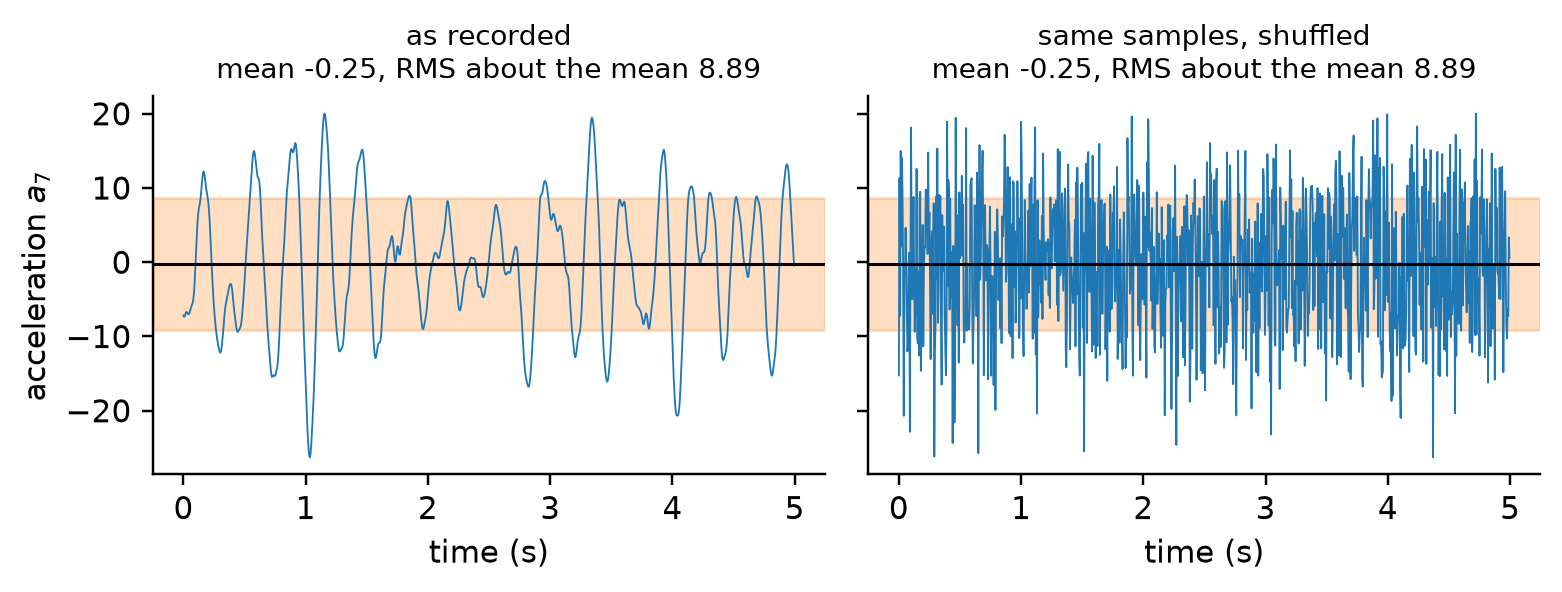
(c) How does it deviate? This is the question the first two cannot touch. The steepest slope in the record, \(\max|\mathrm{d}y/\mathrm{d}t|\), is one answer; how strongly the value now predicts the value a second later is another; and “which frequencies is it made of?” is the answer the rest of this lecture develops. What these summaries share, and what separates them from (a) and (b), is that they depend on the order of the samples. Shuffle a record and its mean, RMS, peak, and every other answer to (a) and (b) are untouched, because they are computed from the collection of values without regard to when each occurred (Figure 7.1). Every answer to (c) is destroyed by the same shuffle. Static summaries are blind to time; dynamic ones are made of it.
Show the code
seg = seis[1600:2600, 6] # channel a7, t = 8 to 13 srng = np.random.default_rng(12778)shuf = rng.permutation(seg)tt = np.arange(len(seg))/fs_casefig, axs = plt.subplots(1, 2, figsize=(7.2, 2.8), sharey=True)for ax, y, ttl in ((axs[0], seg, "as recorded"), (axs[1], shuf, "same samples, shuffled")): m, r = y.mean(), y.std() ax.plot(tt, y, lw=0.6, color="C0") ax.axhline(m, color="k", lw=1); ax.axhspan(m - r, m + r, color="C1", alpha=0.25) ax.set_title(f"{ttl}\nmean {m:.2f}, RMS about the mean {r:.2f}", fontsize=9) ax.set_xlabel("time (s)")axs[0].set_ylabel("acceleration $a_7$")plt.tight_layout(); plt.show()
Figure 7.1: Five seconds of one accelerometer channel from this lecture’s case study (left) and the same samples in a random order (right). Mean and \(\pm\)RMS band — the answers to questions (a) and (b) — are identical for the two records; only a question about how the signal moves in time can tell them apart.
TipActive Learning: Tell them apart
You are given two records of 1000 samples each: a vibration record from a footbridge, and the same record with its samples shuffled into a random order. Using only mean, RMS, minimum, maximum, and any other summary you can compute without looking at the plot, decide which is which. When you conclude that no such summary can tell them apart, name a quantity that could — and notice that every candidate you propose involves the order in which the samples arrived.
One key interesting fact that will support most of the rest of this section is that most signals (even non-deterministic ones) can be approximated via an infinite sum of periodic signals. This view allows us to estimate all of the above properties by analyzing the values of the periodic signals that comprise this approximation: the mean turns out to be the zero-frequency term, the RMS the total size of all the terms together, and the time-evolving behavior — question (c) — the distribution of that size across frequency. Figliola and Beasley’s analogy is a prism: white light in, a spectrum of pure colors out, each color a simple periodic function and its intensity an amplitude (Figliola and Beasley 2019). Fourier analysis is the prism for signals.
7.2.2 Fourier Series
A rectified 60 Hz supply, a footbridge under a marching crowd, and mains hum in a strain-gauge line all repeat, and for a signal that repeats the question “which frequencies does it contain?” has an exact answer. A periodic signal satisfies \(y(t + T) = y(t)\) for some period \(T\), and Fourier’s claim is that any such signal of practical interest can be written as a constant plus a sum of sines and cosines whose frequencies are integer multiples of \(1/T\).
Imagine we have a periodic signal \(y(t)\) with period \(2\pi\), and suppose it can be written as the trigonometric series
The whole question is how to find the coefficients, and the answer rests on three integrals over one period — the orthogonality of sines and cosines: for positive integers \(m\) and \(n\),
where \(\delta_{nm}\) is \(1\) when \(n = m\) and \(0\) otherwise, and every one of these integrands also integrates to zero against a constant. Integrate Equation 7.3 over a period: every sine and cosine term vanishes and \(\int_{-\pi}^{\pi} y\,\mathrm{d}t = 2\pi A_0\). Multiply Equation 7.3 by \(\cos mt\) and integrate: by Equation 7.4 every term dies except the one with \(n = m\), which contributes \(\pi A_m\). The same with \(\sin mt\) picks out \(B_m\). Together these are the Euler formulas,
and the series with these coefficients is the Fourier series of \(y\)(Figliola and Beasley 2019). Each coefficient is a projection: how much of the signal “points along” a given sinusoid, in exactly the sense that a dot product measures how much one vector points along another.
Now imagine we make the period be an arbitrary \(T\). Nothing changes but the scale of time: with the fundamental circular frequency \(\omega = 2\pi/T\) the series and its coefficients become
The \(n = 1\) term is the fundamental, at the lowest frequency in the series, \(f_1 = 1/T\); the terms for \(n = 2, 3, \ldots\) are the harmonics, at exact multiples of it. A sine and a cosine at the same frequency are one sinusoid with a phase, so the series is equally well written with one amplitude and one phase per harmonic,
and a plot of \(C_n\) against \(n f_1\) is the signal’s amplitude spectrum: the prism’s output.
A symmetry shortcut saves half the work. A function is even if \(g(-t) = g(t)\), like \(\cos\), and odd if \(h(-t) = -h(t)\), like \(\sin\). The product of an even function with an odd one is odd, and an odd function integrates to zero over a symmetric interval, so an even signal has \(B_n = 0\) for every \(n\) — a cosine series — and an odd signal has \(A_0 = A_n = 0\) — a sine series. A signal that is neither needs both. The rectified sine of a power supply is even, so its series is cosines only; the square wave below is odd, so it is sines only.
Take Figliola and Beasley’s square wave, \(y(t) = -5\) for \(-\pi < t < 0\) and \(+5\) for \(0 < t < \pi\), repeating with period \(2\pi\). It is odd, so only the \(B_n\) survive, and by Equation 7.5
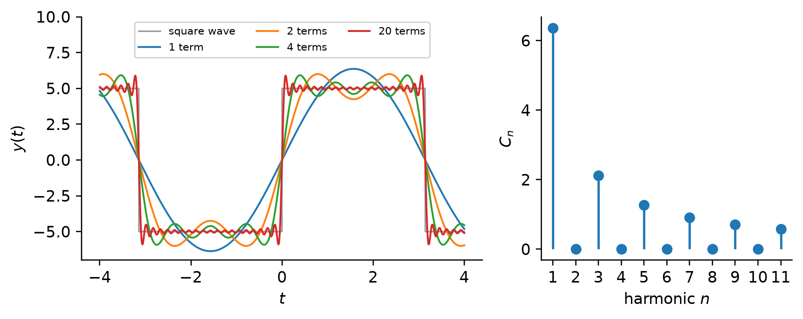
so that \(y(t) = \frac{20}{\pi}\left(\sin t + \tfrac{1}{3}\sin 3t + \tfrac{1}{5}\sin 5t + \cdots\right)\). Only odd harmonics, with amplitudes falling as \(1/n\): the spectrum of a square wave is a picket fence with every other picket missing. Figure 7.2 shows the partial sums closing in on the waveform — and one detail worth remembering when we get to leakage: the jump is the hard part. A discontinuity needs infinitely many harmonics, and every truncated series overshoots at the edge, however many terms are kept.
Figure 7.2: Left: the \(\pm 5\) square wave and the partial sums of its Fourier series with one, two, four, and twenty terms. Each added harmonic sharpens the edges but the overshoot at the jump never goes away. Right: the amplitude spectrum, \(C_n = 20/(n\pi)\) at odd \(n\) and zero at even \(n\).
Build the square wave yourself: the slider sets how many odd harmonics are kept.
viewof nharm = Inputs.range([1,41], {value:3,step:2,label:"highest harmonic n kept"})
squarePlot = {const pts = [];for (let i =0; i <=600; i++) {const t =-4+8* i /600;let y =0;for (let n =1; n <= nharm; n +=2) y +=20/ (n *Math.PI) *Math.sin(n * t); pts.push({t, y,kind:"partial sum"}); pts.push({t,y:5*Math.sign(Math.sin(t) ||1e-9),kind:"square wave"}); }const spec = [];for (let n =1; n <=41; n++) spec.push({n,C: n %2?20/ (n *Math.PI) :0,kept: n <= nharm ?"kept":"dropped"});returnhtml`<div style="font-family:sans-serif">${Plot.plot({width:640,height:220,x: {label:"t"},y: {label:"y(t)",domain: [-7,7]},color: {legend:true,domain: ["square wave","partial sum"],range: ["#bbb","steelblue"]},marks: [Plot.line(pts, {x:"t",y:"y",stroke:"kind",z:"kind"})]})}${Plot.plot({width:640,height:160,x: {label:"harmonic n",domain: [0,42]},y: {label:"C_n"},color: {legend:true,domain: ["kept","dropped"],range: ["steelblue","#ddd"]},marks: [Plot.ruleX(spec, {x:"n",y:"C",stroke:"kept",strokeWidth:2.5})]})}</div>`;}
7.2.3 From Series to Transform
Now let’s imagine (as is the case in practice, mostly) that we don’t know the actual period of the signal we are measuring. The most that this period could be would be infinity — a signal that never repeats is one whose period is infinite — so the natural question is what happens to the series when \(T\) is taken to that limit. Letting the period grow without bound turns the sum of harmonics into an integral over every frequency, and the coefficients into a single complex function \(Y(\omega)\) whose magnitude says how much of each sinusoid is present and whose phase says where it sits in time.
Start from Equation 7.7 and pull the \(2/T\) outside: \(A_n = (2/T)\,A_T(n\omega)\) with \(A_T(\omega') = \int_{-T/2}^{T/2} y(t)\cos\omega' t\,\mathrm{d}t\), and likewise for \(B_n\). Since \(2/T = \omega/\pi\), the series Equation 7.6 reads
As \(T \to \infty\) three things happen at once: the harmonic spacing \(\omega = 2\pi/T\) shrinks toward an infinitesimal \(\mathrm{d}\omega\); the harmonic frequencies \(n\omega\) fill in every value of a continuous \(\omega\); and the sum, which has the form \(\sum g(n\omega)\,\omega\), becomes the integral \(\int g(\omega)\,\mathrm{d}\omega\). (The constant \(A_0\) goes to zero for any pulse of finite energy, since it is a finite integral divided by \(T\).) The Fourier coefficients\(A_n\) and \(B_n\) have become continuous functions of frequency,
and the signal is recovered from them as \(y(t) = \frac{1}{\pi}\int_0^{\infty}\left[A(\omega)\cos\omega t + B(\omega)\sin\omega t\right]\mathrm{d}\omega\). Two real functions are one complex function, and Euler’s identity \(e^{-j\theta} = \cos\theta - j\sin\theta\) (with \(j = \sqrt{-1}\), the engineer’s letter, since \(i\) is a current) packs the pair into the Fourier transform
For a real signal \(Y(-\omega)\) is the complex conjugate of \(Y(\omega)\), which lets the recovery integral run over negative frequencies too and absorb the sine and cosine into one exponential. Written in hertz, with \(\omega = 2\pi f\), the pair is
\[
Y(f) = \int_{-\infty}^{\infty} y(t)\,e^{-j2\pi f t}\,\mathrm{d}t,
\qquad
y(t) = \int_{-\infty}^{\infty} Y(f)\,e^{+j2\pi f t}\,\mathrm{d}f,
\tag{7.12}\]
the forward transform and the inverse Fourier transform, and with \(f\) as the variable no stray factors of \(2\pi\) appear anywhere. The transform is two-sided — it runs over negative frequencies as well — and for a real signal the negative half is the mirror image of the positive half, so it carries no new information; plots show \(f \geq 0\).
What is \(Y(f)\)? At each frequency it is a complex number, and its polar form is the useful one:
The magnitude\(|Y(f)|\) is the amplitude spectrum of Equation 7.8 with the pickets pushed together into a continuous curve: how much of the sinusoid at \(f\) the signal contains. The phase\(\phi(f)\) says where that sinusoid sits in time — shift the whole signal later by \(t_0\) and every \(|Y(f)|\) is unchanged while every phase turns by \(-2\pi f t_0\). A signal is, in other words, described exactly as well by \(Y(f)\) as by \(y(t)\); the transform is a change of point of view, not a loss of information, and it is the point of view from which Lecture 5’s filters and this lecture’s structures are easy to read.
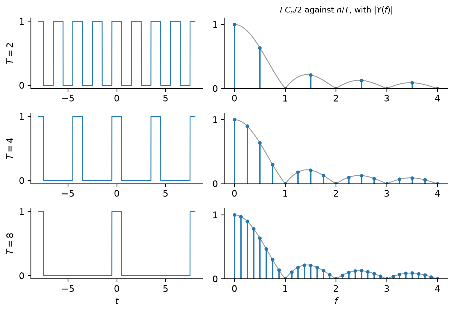
Figure 7.3 shows the limit at work on a rectangular pulse. Repeated with period \(T\), the pulse has a line spectrum whose pickets sit \(1/T\) apart and whose heights, scaled by \(T\), all lie on one curve. Double the period and the pickets crowd twice as densely under the same curve; the curve is \(|Y(f)|\), the transform of the single pulse, and the pickets are its samples.
Show the code
tau =1.0fig, axs = plt.subplots(3, 2, figsize=(7.2, 5.0), gridspec_kw={"width_ratios": [1, 1.3]})ff = np.linspace(0, 4, 800)Ycont = tau*np.abs(np.sinc(ff*tau)) # |Y(f)| of the single pulse (numpy's sinc is sin(pi x)/(pi x))for row, T inzip(axs, (2, 4, 8)): tt = np.linspace(-8, 8, 3200) pulse = (np.abs((tt + T/2) % T - T/2) <= tau/2).astype(float) row[0].plot(tt, pulse, lw=1); row[0].set_yticks([0, 1]); row[0].set_ylabel(f"$T = {T}$") nn = np.arange(1, int(4*T) +1) An_ = (2/T)*tau*np.sinc(nn*tau/T) # cosine coefficients of the even pulse train row[1].plot(ff, Ycont, color="0.6", lw=1) row[1].stem(nn/T, T*np.abs(An_)/2, basefmt=" ", markerfmt="C0.", linefmt="C0-") row[1].stem([0], [T*tau/T], basefmt=" ", markerfmt="C0.", linefmt="C0-") row[1].set_ylim(0, 1.1); row[1].set_yticks([0, 1])axs[-1][0].set_xlabel("$t$"); axs[-1][1].set_xlabel("$f$")axs[0][1].set_title("$T\\,C_n / 2$ against $n/T$, with $|Y(f)|$", fontsize=9)plt.tight_layout(); plt.show()
Figure 7.3: A rectangular pulse of unit width and height repeated with period \(T = 2\), \(4\), and \(8\) (left) and its Fourier coefficients scaled by \(T\) (right, stems). As the period grows the harmonics crowd together, and all of them lie on the transform of the single pulse (curve): the series becomes the transform.
CautionConcept Check: Pickets and curves
A periodic signal has period \(T = 0.5\) s. Where are its harmonics on the frequency axis, and what happens to that picture if the period is doubled, then doubled again, then made infinite?
TipAnswer
The harmonics sit at multiples of \(1/T = 2\) Hz: \(2, 4, 6, \ldots\) Hz. Doubling \(T\) to 1 s puts them 1 Hz apart, and to 2 s puts them 0.5 Hz apart — the pickets crowd together, and (scaled by \(T\)) they keep lying on the same curve. In the limit of infinite period the pickets are dense on the axis and the curve itself, \(|Y(f)|\), is the description: the Fourier transform is not a different tool from the series but its limit, which is why a signal that does not repeat still has a spectrum.
7.3 The DFT and Its Bins
In practice, we will be computing this transform on a discrete signal \(y[n]\) given that we will apply it after the ADC has digitized the signals from the sensors. Thus, we need a discrete version of the transform — and the version we get carries a fine print about periodicity that is the source of every practical difficulty in the rest of the lecture.
Start from the forward transform in Equation 7.12 and make it computable. The record is \(N\) samples, \(y[n] = y(n\,\delta t)\) for \(n = 0, \ldots, N-1\), so the integral becomes a sum with \(\mathrm{d}t \to \delta t\) and \(t \to n\,\delta t\). The record is finite, so the transform can only be asked about frequencies that fit a whole number of cycles into it — \(f_k = k/(N\,\delta t)\), or equivalently \(k\,f_s/N\), for integer \(k\). Substituting both, \(e^{-j2\pi f_k n\,\delta t} = e^{-j2\pi kn/N}\), and dropping the overall factor \(\delta t\) (a convention; it only scales the result), we have the discrete Fourier transform
\(N\) numbers in, \(N\) complex numbers out, and Equation 7.15 says nothing was lost: the \(N\) values \(Y[k]\) are just another set of coordinates for the same record, exactly as \(Y(f)\) was for \(y(t)\). This is the convention NumPy’s fft uses, and the one we adopt; Figliola and Beasley’s version divides by \(N/2\) so that the result reads directly in amplitude, which is the scaling in Equation 7.17 below (Figliola and Beasley 2019).
What did this do to our assumption of an infinite period? It threw it away. The exponential \(e^{-j2\pi kn/N}\) repeats every \(N\) samples, so the only signals Equation 7.15 can build are ones that repeat every \(N\) samples — the DFT treats your \(N\) samples as one period of a periodic signal of period \(N\,\delta t\), whether or not the physical signal ever repeated. This is the fine print. It is also the reason the frequencies come out where they do: the lowest nonzero frequency the DFT can distinguish is one full cycle per record,
\[
\delta f = \frac{1}{N\,\delta t} = \frac{f_s}{N},
\tag{7.16}\]
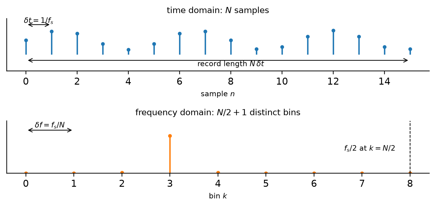
Lecture 4’s frequency resolution (Equation 5.5), now with its origin visible. Resolution is bought with record length, \(N\,\delta t\), and with nothing else: sampling faster with the same \(N\) shortens the record and makes \(\delta f\) coarser, not finer (Figure 7.4). Three of the \(N\) bins deserve names. Bin \(k = 0\) is \(Y[0] = \sum y[n] = N\bar{y}\), the mean of Equation 7.1 scaled by \(N\) — the static component, question (a), is the first coefficient of the spectrum. Bin \(k = N/2\) (for even \(N\)) sits at \(f_s/2\), the Nyquist frequency. And the bins above \(N/2\) are the negative frequencies in disguise: for a real record \(Y[N-k]\) is the complex conjugate of \(Y[k]\), the mirror image Lecture 5 saw in the replica picture, so the upper half repeats the lower half and NumPy’s rfft simply omits it. Reading an amplitude off the lower half requires the scaling
\[
C_k = \frac{2}{N}\,|Y[k]|,\qquad 0 < k < \frac{N}{2},
\tag{7.17}\]
the factor \(2\) collecting the mirror bin’s share and the \(1/N\) undoing the sum’s growth with record length — this is the amplitude \(C_n\) of Equation 7.8, for the harmonic that fits \(k\) cycles into the record.
Figure 7.4: The four quantities to keep straight. A record of \(N\) samples spaced \(\delta t = 1/f_s\) lasts \(N\,\delta t\) (top); its DFT has bins spaced \(\delta f = f_s/N\) apart, running from 0 to the Nyquist frequency \(f_s/2\) at bin \(N/2\) (bottom). Doubling \(f_s\) with \(N\) fixed halves the record and doubles \(\delta f\).
CautionConcept Check: Faster, not finer
You keep \(N\) fixed at 1024 samples and double the sampling rate from 100 to 200 Hz. Does the frequency resolution of your DFT improve?
TipAnswer
No — it gets worse. By Equation 7.16, \(\delta f = f_s/N\) goes from about 0.098 Hz to 0.195 Hz, because the record now lasts 5.12 s instead of 10.24 s and the lowest frequency that fits one cycle into it has doubled. What the higher rate bought is range: the Nyquist frequency moved from 50 to 100 Hz. Resolution comes from record length, range from sampling rate, and only more samples can buy both.
7.3.1 Bin Index to Hertz
A call to numpy.fft.fft returns a list of \(N\) complex numbers indexed from 0 to \(N-1\), and nothing in that list says hertz. The conversion is the one we just derived, \(f_k = k\,f_s/N\), and a worked example makes it concrete: a sinusoid of 120 Hz and unit amplitude, sampled at 360 Hz. (120 Hz is the fundamental of a full-wave-rectified 60 Hz supply and the flicker frequency of mains-powered lamps — it turns up uninvited in a great many lab records, including the one Lecture 5’s exercises aliased to DC.)
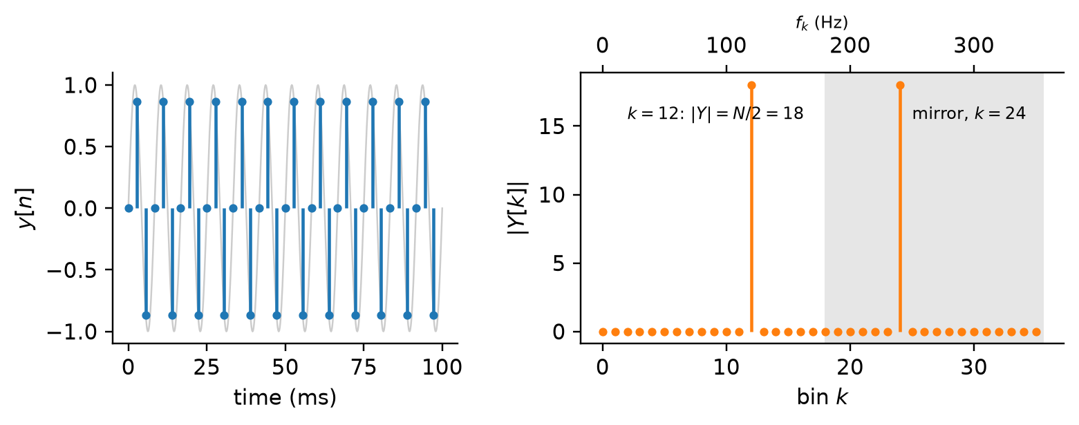
Three samples per cycle, since \(360/120 = 3\), so the sampled tone takes only three distinct values, \(\sin(0)\), \(\sin(2\pi/3)\), and \(\sin(4\pi/3)\) — that is, \(0\), \(0.866\), and \(-0.866\) — over and over. For the tone to land on a bin the record must hold a whole number of cycles, so \(N\) must be a multiple of 3; take \(N = 36\), a tenth of a second. Then \(\delta f = 360/36 = 10\) Hz and the tone falls at \(k = 120/10 = 12\), exactly. Figure 7.5 shows the result: \(|Y[12]| = 18 = N/2\), its mirror at \(k = 24\) (that is, \(N - 12\)), and nothing anywhere else. The amplitude scaling of Equation 7.17 gives \(C_{12} = 2 \times 18/36 = 1\), the amplitude we started with.
Figure 7.5: The DFT of a unit-amplitude 120 Hz tone sampled at 360 Hz for \(N = 36\) samples. Left: the record — only three distinct sample values. Right: \(|Y[k]|\) against bin index (bottom axis) and against \(f_k = k f_s / N\) (top axis). The tone lands entirely in bin 12, with its mirror image in bin \(N - 12 = 24\); the shaded half above \(N/2\) carries no new information.
Computing Equation 7.14 literally costs \(N\) multiplications for each of \(N\) bins, \(N^2\) in all, which for a one-second record at 200 kS/s is \(4 \times 10^{10}\) operations — too slow to be routine in 1965 and too slow for real-time instruments today. The fast Fourier transform (FFT) is an algorithm, published by Cooley and Tukey, that computes exactly the same \(N\) numbers in about \(N \log_2 N\) operations by splitting the sum recursively into even- and odd-indexed halves (Cooley and Tukey 1965). For \(N = 2^{20}\) (about a million samples) the saving is a factor of \(N/\log_2 N \approx 52{,}000\), which is the difference between minutes and milliseconds — and the reason spectral analysis went from a specialist’s calculation to a function call. Its one habit worth knowing is a preference for \(N\) that is a power of 2, which is why records are often padded or truncated to \(1024\), \(4096\), and so on. The FFT is not a different transform: numpy.fft.fft returns Equation 7.14 to within rounding error, for any \(N\).
7.4 Leakage and Windows
Since our assumption after the DFT is that the signals are periodic, we need to be careful about how we interpret the results if we are only carrying out the analysis on a subset (a window) of the full signal we’re measuring. Unless the record holds a whole number of cycles of every component in it, its periodic extension has a jump at the seam, and that jump smears energy into neighboring bins — leakage — so that a pure tone reads as a smaller peak with a skirt. Tapering the record with a window softens the seam, trading a little resolution for much less smearing.
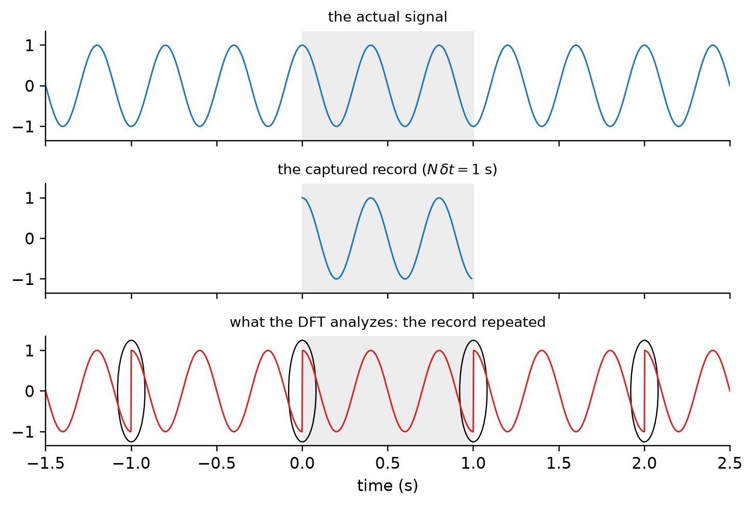
Figure 7.6 draws the assumption the DFT makes without asking. The signal continues before and after the record (top); we captured a finite piece of it (middle); and Equation 7.15 describes not that piece but the piece repeated end to end forever (bottom). If the record held a whole number of cycles the copies would join seamlessly and the extension would be the original signal. Here it does not, and at every seam the extended signal jumps from the last sample’s value to the first’s — a discontinuity the physical signal never had.
Show the code
fpe, fs_pe, Tpe =2.5, 100, 1.0tt = np.linspace(-1.5, 2.5, 2000)tr = np.arange(0, Tpe, 1/fs_pe)fig, axs = plt.subplots(3, 1, figsize=(6.8, 4.6), sharex=True)axs[0].plot(tt, np.cos(2*np.pi*fpe*tt), lw=1); axs[0].set_title("the actual signal", fontsize=9)axs[1].plot(tr, np.cos(2*np.pi*fpe*tr), lw=1); axs[1].set_xlim(-1.5, 2.5); axs[1].set_title("the captured record ($N\\,\\delta t = 1$ s)", fontsize=9)ext = np.cos(2*np.pi*fpe*(tt % Tpe))axs[2].plot(tt, ext, lw=1, color="C3"); axs[2].set_title("what the DFT analyzes: the record repeated", fontsize=9)from matplotlib.patches import Ellipsefor s in (-1, 0, 1, 2): axs[2].add_patch(Ellipse((s, 0), width=0.16, height=2.5, fill=False, color="k", lw=0.8))for ax in axs: ax.set_yticks([-1, 0, 1]); ax.set_ylim(-1.35, 1.35); ax.axvspan(0, Tpe, color="0.93", zorder=0)axs[2].set_xlabel("time (s)")plt.tight_layout(); plt.show()
Figure 7.6: What the DFT assumes. Top: the actual signal, a 2.5 Hz cosine that continues indefinitely. Middle: the one-second record we captured, holding two and a half cycles. Bottom: the periodic extension the DFT analyzes — the record repeated end to end — with a jump from \(-1\) to \(+1\) at every seam (circled) that the real signal never contained.
Why should a jump at the seam trouble the spectrum? Because the square wave already told us: a discontinuity is the most expensive feature a Fourier series can represent, needing every harmonic with amplitudes that decay only as \(1/n\) (Equation 7.9). The DFT of the extended signal must therefore spend energy on harmonics the true signal never contained, and it takes that energy from the tone’s own bin. The tone’s peak comes out lower than the truth and a skirt of spurious content spreads to either side — content that leaked out of the bin it belonged in. The same mechanism is responsible for Lecture 4’s amplitude ambiguity (Figure 5.4), which we can now state precisely: the DFT reports a tone’s amplitude correctly only when the tone fits a whole number of cycles into the record.
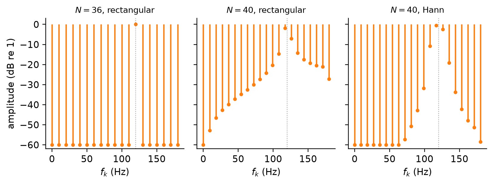
Return to the 120 Hz tone, and change one thing: sample \(N = 40\) points instead of 36. Now \(\delta f = 9\) Hz, and 120 Hz sits between bins 13 (117 Hz) and 14 (126 Hz) — the record holds \(13\tfrac{1}{3}\) cycles. Figure 7.7 shows the damage: the largest bin reads an amplitude of \(0.80\) instead of \(1\), its neighbor reads \(0.44\), and every bin above dc is nonzero. About 11% of the tone’s energy has left the immediate neighborhood of its true frequency.
The remedy is to soften the seam before transforming. A window\(w[n]\) is a sequence that is \(1\) in the middle of the record and tapers smoothly to \(0\) at both ends; multiply the record by it,
\[
y_w[n] = w[n]\,y[n],
\tag{7.18}\]
and the periodic extension of \(y_w\) now joins gently at every seam, because both ends have been brought to zero. The unwindowed DFT is itself the windowed DFT with the rectangular window — all ones — so the choice is never whether to window, only which window. The workhorse is the Hann window, \(w[n] = \tfrac{1}{2}\left[1 - \cos\!\big(2\pi n/(N-1)\big)\right]\), a raised cosine. Figure 7.7 shows what it does to the \(N = 40\) record: the skirt collapses by an order of magnitude and the leaked energy outside the tone’s neighborhood falls from 11% to under 1%, at the price of a peak that is now two bins wide rather than one. (The window also scales the record — it averages \(\tfrac{1}{2}\) — so amplitudes read from a Hann-windowed spectrum are multiplied by 2, or in general divided by the window’s mean.)
Show the code
def amp_spectrum(y, w): A = np.abs(np.fft.rfft(y*w))/w.sum() # corrected for the window's mean A[1:(len(y) +1)//2] *=2# fold in the mirror bins, 0 < k < N/2 (@eq-dft-amp); dc and Nyquist have nonereturn Acases = [("$N = 36$, rectangular", 36, "rect"), ("$N = 40$, rectangular", 40, "rect"), ("$N = 40$, Hann", 40, "hann")]fig, axs = plt.subplots(1, 3, figsize=(7.6, 2.9), sharey=True)for ax, (ttl, N_, kind) inzip(axs, cases): n_ = np.arange(N_); y_ = np.sin(2*np.pi*f120*n_/fs120) w_ = np.ones(N_) if kind =="rect"else np.hanning(N_) A_ = amp_spectrum(y_, w_); fk = np.fft.rfftfreq(N_, 1/fs120) ax.stem(fk, np.maximum(dB(A_ +1e-12), -60), basefmt=" ", markerfmt="C1.", linefmt="C1-") ax.axvline(120, color="0.6", ls=":", lw=0.8); ax.set_title(ttl, fontsize=9); ax.set_xlabel("$f_k$ (Hz)")axs[0].set_ylabel("amplitude (dB re 1)"); axs[0].set_ylim(-62, 3)plt.tight_layout(); plt.show()
Figure 7.7: Leakage and its remedy, for the 120 Hz tone sampled at 360 Hz. Left: \(N = 36\) holds twelve whole cycles and the tone lands entirely in one bin. Middle: \(N = 40\) holds \(13\tfrac{1}{3}\) cycles, and the tone’s energy spreads across every bin above dc — the peak reads 0.80 instead of 1. Right: the same 40 samples multiplied by a Hann window before the DFT; the skirt drops by an order of magnitude and the peak widens to two bins. Amplitudes are shown on a decibel scale relative to a unit tone.
What kind of operation is windowing? It is linear — window a sum and you get the sum of the windowed records — but it is not time-invariant: slide the record by ten samples and the taper falls on different samples, so windowing is a time-varying gain and not one of Lecture 5’s LTI blocks (Section 6.2.1). Its natural description is the mirror image of a filter’s. A filter convolves in time and multiplies in frequency; a window multiplies in time, Equation 7.18, and therefore convolves in frequency,
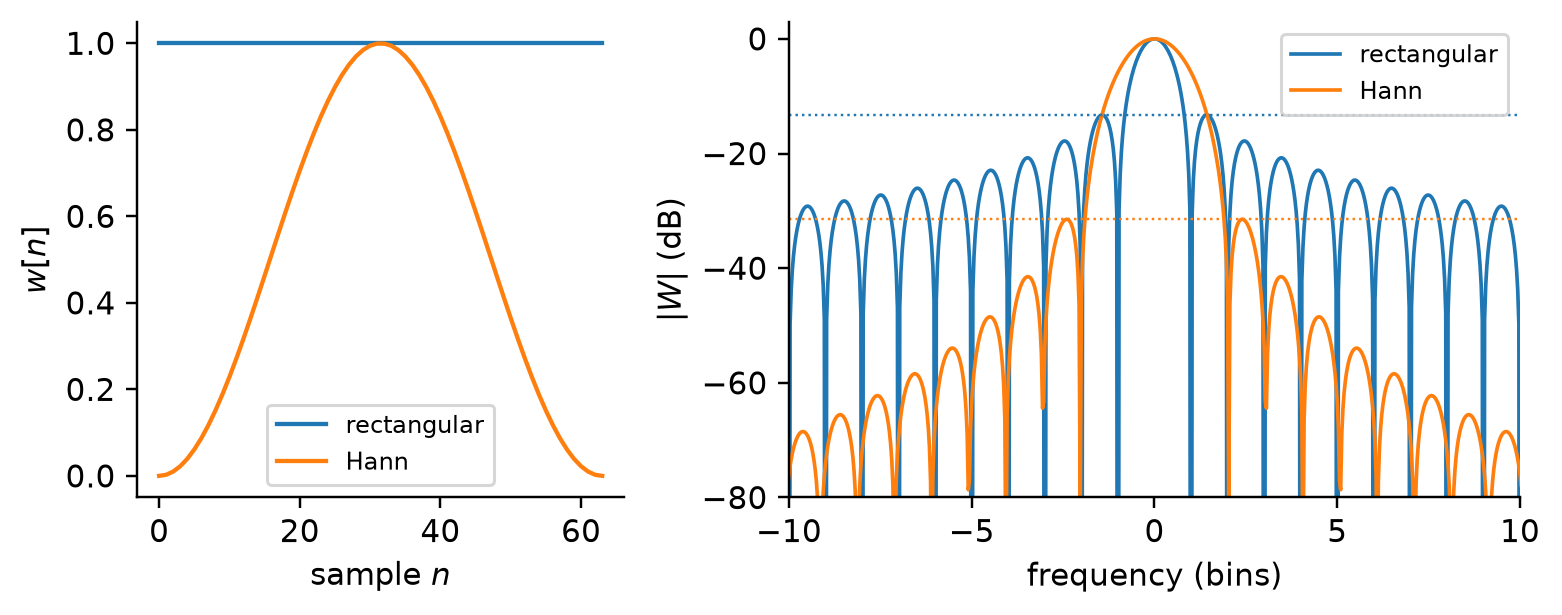
where \(W\) is the window’s own transform. Every line in the true spectrum is replaced by a copy of \(W\) centered on it, so the spectrum you measure is the true spectrum seen through the window’s transform, and choosing a window means choosing the shape of \(W\) (Figure 7.8). The rectangular window’s \(W\) has a narrow main lobe — good resolution — but side lobes only 13 dB down that decay slowly, which is the skirt in Figure 7.7. The Hann window’s main lobe is twice as wide, and its first side lobe is 31 dB down and the rest fall away quickly. That is the whole trade: a narrow main lobe resolves close tones, low side lobes stop a strong tone from burying a weak one, and no window has both, which is why the catalog of windows runs to dozens (Harris 1978). For finding modal peaks in vibration data, the Hann window is the default and is rarely wrong.
Figure 7.8: Two windows and their transforms. Left: the rectangular window (all ones) and the Hann window in time. Right: \(|W(f)|\) for each, in decibels against frequency in units of bins (\(\delta f\)). The rectangular window has the narrower main lobe (nulls at \(\pm 1\) bin) but side lobes only 13 dB down; the Hann window’s main lobe is twice as wide (first null near \(\pm 2\) bins) and its side lobes start 31 dB down and fall fast. This transform is what every spectral line is convolved with.
Try it: the 120 Hz tone at \(f_s = 360\) Hz again, with the record length and the window under your control. Watch what happens to the peak and to the skirt as \(N\) passes through multiples of 3.
leakPlot = {const fs =360, f0 =120, N = leak.N;const w =Array.from({length: N}, (_, n) => leak.hann?0.5* (1-Math.cos(2*Math.PI* n / (N -1))) :1);const y =Array.from({length: N}, (_, n) =>Math.sin(2*Math.PI* f0 * n / fs) * w[n]);const wsum = w.reduce((s, v) => s + v,0);const spec = [];for (let k =0; k <= N /2; k++) {let re =0, im =0;for (let n =0; n < N; n++) { re += y[n] *Math.cos(2*Math.PI* k * n / N); im -= y[n] *Math.sin(2*Math.PI* k * n / N); }const A = (k >0&&2* k < N ?2:1) *Math.hypot(re, im) / wsum;// dc and Nyquist bins have no mirror spec.push({f: k * fs / N,A:Math.max(20*Math.log10(A +1e-12),-60)}); }const cycles = f0 * N / fs, whole =Math.abs(cycles -Math.round(cycles)) <1e-9;const peak = spec.reduce((m, o) => o.A> m.A? o : m, spec[0]);returnhtml`<div style="font-family:sans-serif"><b>δf = ${(fs / N).toFixed(2)} Hz</b> · the record holds ${cycles.toFixed(2)} cycles${whole ?" — a whole number: no leakage":" — not a whole number: leakage"} · largest bin at ${peak.f.toFixed(1)} Hz reads ${Math.pow(10, peak.A/20).toFixed(2)}${Plot.plot({width:640,height:220,x: {label:"f_k (Hz)",domain: [0,180]},y: {label:"amplitude (dB re 1)",domain: [-62,3]},marks: [Plot.ruleX([f0], {stroke:"#999",strokeDasharray:"3,3"}), Plot.ruleX(spec, {x:"f",y1:-62,y2:"A",stroke:"darkorange",strokeWidth:2}), Plot.dot(spec, {x:"f",y:"A",fill:"darkorange",r:2.5})]})}</div>`;}
TipActive Learning: Predict before you plot
Set the widget above (or the code in Figure 7.7) aside for a moment. The 120 Hz tone is sampled at 360 Hz for \(N = 42\) samples, then for \(N = 44\). For each, say before computing whether the tone lands on a bin, which bin or pair of bins it falls nearest, and what amplitude the largest bin will read — then check. Explain, in one sentence each, what \(N = 42\) has in common with \(N = 36\), and why \(N = 44\) leaks about as badly as \(N = 40\) despite being the longer record.
CautionConcept Check: Does the window remove leakage?
A colleague says that applying a Hann window “removes the leakage” from a spectrum. Is that right?
TipAnswer
Not quite: it redistributes it. By Equation 7.19 every spectral line is convolved with the window’s transform, and the Hann window’s transform has a main lobe twice as wide as the rectangular window’s. The far skirt drops by tens of decibels, but the energy near the tone spreads over two bins instead of one — resolution is traded for side-lobe suppression. The only way to have no leakage at all is a record holding a whole number of cycles of every component, which for real data with unknown frequencies never happens.
NoteOptional: Power Spectral Density
This section is optional: it is not among the lecture’s learning objectives, and nothing after it depends on it. Read it when you meet a signal — wind, traffic, machinery — that never settles into a repeating pattern and you need a spectrum of the process rather than of one record.
For a nondeterministic signal — traffic-induced vibration of a bridge deck, wind pressure on a façade — the DFT magnitude of a single record never settles down no matter how long the record, so we need a spectrum that describes the process rather than one realization of it. The power spectral density tells how the signal’s variance is distributed over frequency; it is estimated by averaging the periodograms of windowed segments (Welch’s method), and its integral is the variance — the RMS from Section 7.2, now resolved by frequency.
Everything so far took the signal to be deterministic: a tone has an amplitude, and a longer record pins it down more finely. A random signal has no amplitude at any frequency; it has a distribution of amplitudes, and what is fixed — for a stationary process, one whose statistics do not drift over the record — is the average power at each frequency. The natural estimator is the squared DFT, scaled so that it integrates to the variance: the periodogram
with units of (signal units)\(^2\) per hertz — acceleration in \((\mathrm{m/s^2})^2/\mathrm{Hz}\), pressure in \(\mathrm{Pa^2/Hz}\) — so that the area under it between two frequencies is the variance contributed by that band. (The factor 2 folds the mirror half in, as in Equation 7.17; the dc bin and the Nyquist bin get half of it.) That the area is the variance is Parseval’s theorem,
energy in the time domain equals energy in the frequency domain: for a zero-mean record, dividing both sides by \(N\) makes the left the variance, \(y_{\mathrm{rms}}^2\) of Equation 7.2, and the right the sum of the periodogram times \(\delta f\). So the RMS is the square root of the area under the PSD — question (b) again — and the PSD is what question (c) adds: where on the frequency axis that area sits.
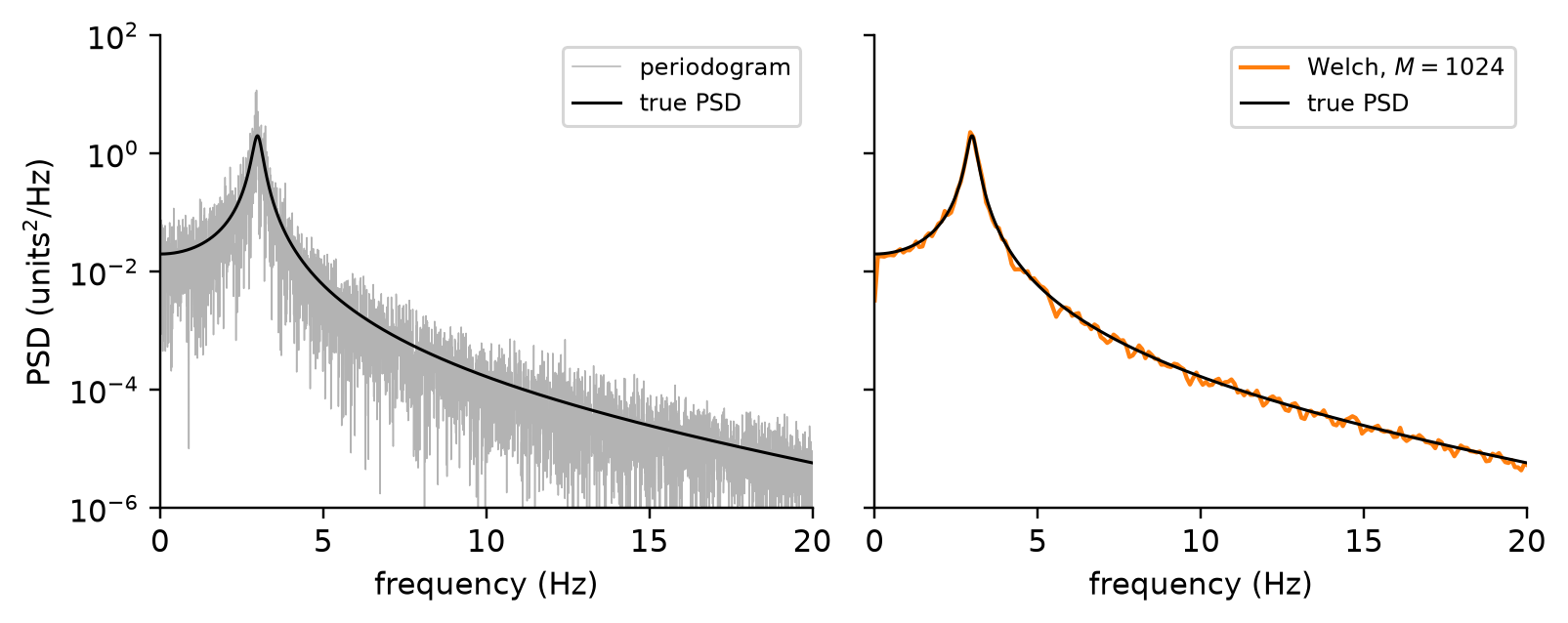
The periodogram has one crippling defect. Each of its bins is, for a random signal, an estimate from what amounts to one sample, and its scatter is as large as its mean regardless of \(N\): a longer record gives more bins, each as noisy as before. The left panel of Figure 7.9 shows it — a spectrum that looks like grass. Welch’s remedy is to spend the record on averaging rather than on resolution (Welch 1967). Split the \(N\) samples into \(L\) segments of length \(M\) (overlapping by half, which recovers some of what the window taper throws away), window each segment, compute its periodogram, and average:
\[
\hat{S}_W[k] = \frac{1}{L}\sum_{\ell=1}^{L}\hat{S}_\ell[k],\qquad \delta f = \frac{f_s}{M}.
\tag{7.22}\]
The scatter of the average falls as \(1/\sqrt{L}\), and the price is resolution: \(\delta f\) is now \(f_s/M\), not \(f_s/N\). Choosing \(M\) is choosing where to stand between a spectrum too noisy to read and one too coarse to resolve the peaks you care about. SciPy’s signal.welch implements exactly this, with a Hann window and 50% overlap by default; you supply \(M\) as nperseg.
The example in Figure 7.9 is a building mode: a lightly damped oscillator at 3 Hz driven by broadband (white) excitation, sampled at 100 Hz for 200 s. Its true PSD is known — it is the excitation’s flat spectrum shaped by the oscillator’s frequency response, a peak at 3 Hz whose half-power width is \(2\zeta f_n = 0.3\) Hz for 5% damping. The periodogram scatters around it wildly; the Welch estimate with \(M = 1024\) (\(\delta f \approx 0.1\) Hz, 38 segments) follows it closely and still resolves the peak. And the areas agree: the Welch estimate integrates to the record’s variance to within 1%.
Show the code
fs_ex, fn_ex, zeta_ex =100, 3.0, 0.05wn =2*np.pi*fn_exb_ex, a_ex = signal.bilinear([wn**2], [1, 2*zeta_ex*wn, wn**2], fs_ex) # the oscillator as a digital filterrng_ex = np.random.default_rng(1)x_ex = signal.lfilter(b_ex, a_ex, rng_ex.normal(0, 1, 20000)) # 200 s of response to unit white noisef_p, S_p = signal.periodogram(x_ex, fs=fs_ex)f_w, S_w = signal.welch(x_ex, fs=fs_ex, nperseg=1024)f_t = np.linspace(0.01, 50, 5000); _, H_t = signal.freqz(b_ex, a_ex, worN=f_t, fs=fs_ex)S_t =2*np.abs(H_t)**2/fs_ex # true one-sided PSD: white input shaped by |H|^2fig, (a1, a2) = plt.subplots(1, 2, figsize=(7.4, 3.0), sharey=True)a1.semilogy(f_p, S_p, color="0.7", lw=0.5, label="periodogram"); a1.semilogy(f_t, S_t, "k", lw=1, label="true PSD")a2.semilogy(f_w, S_w, "C1", lw=1.4, label="Welch, $M = 1024$"); a2.semilogy(f_t, S_t, "k", lw=1, label="true PSD")for ax in (a1, a2): ax.set_xlim(0, 20); ax.set_xlabel("frequency (Hz)"); ax.legend(fontsize=8)a1.set_ylabel("PSD (units$^2$/Hz)"); a1.set_ylim(1e-6, 1e2)plt.tight_layout(); plt.show()
Figure 7.9: Estimating the PSD of a stationary signal — a 3 Hz, 5%-damped mode driven by white noise, sampled at 100 Hz for 200 s. Left: the periodogram of the whole record (grey) scatters around the true PSD (black) by a factor comparable to its own value, and would do so for any record length. Right: Welch’s average of 38 half-overlapping Hann-windowed segments of 1024 samples follows the true PSD; its area, the variance, matches the record’s to within 1%.
Two habits keep PSDs honest. First, subtract the mean before estimating: a dc offset is a spike at \(f = 0\) whose leakage can bury the low-frequency content you want. Second, read the units: a PSD in \((\mathrm{m/s^2})^2/\mathrm{Hz}\) is not an amplitude, and comparing “peak heights” across records with different \(\delta f\) is meaningless unless both are densities. Integrate over a band and take the square root, and you have an RMS in \(\mathrm{m/s^2}\) that can be compared with anything.
ImportantExercise: RMS from a PSD
The PSD of a floor’s vertical acceleration is flat at \(2 \times 10^{-4}\ (\mathrm{m/s^2})^2/\mathrm{Hz}\) from 1 to 4 Hz and at \(5 \times 10^{-5}\ (\mathrm{m/s^2})^2/\mathrm{Hz}\) from 4 to 10 Hz, and negligible elsewhere. The specification limits the RMS acceleration in the 1–10 Hz band to \(0.05\ \mathrm{m/s^2}\). Does the floor comply?
TipSolution
The variance is the area: \(2 \times 10^{-4} \times 3 + 5 \times 10^{-5} \times 6 = 6 \times 10^{-4} + 3 \times 10^{-4} = 9 \times 10^{-4}\ (\mathrm{m/s^2})^2\), so the RMS is \(\sqrt{9 \times 10^{-4}} = 0.030\ \mathrm{m/s^2}\), below the limit. Note that two-thirds of the variance comes from the lower band even though it is half as wide — density times bandwidth, not density alone, is what counts.
7.5 LTI Systems in the Frequency Domain
Lecture 5 drew the Bode plot of an RC filter but never said how to compute what that filter does to an entire measured signal, only to one sinusoid at a time. Now that we can compute \(Y(\omega)\) for any signal \(y(t)\), every block in the measurement chain becomes a multiplication in the frequency domain, which makes it easy to reason about how the chain affects the magnitude and phase of each frequency component throughout.
Recall from Section 6.2.1 that an LTI block is described by its impulse response \(h(t)\), and that its output for any input is the convolution \(y_{\mathrm{out}}(t) = \int h(\tau)\,y(t - \tau)\,\mathrm{d}\tau\) — every input sample launches a scaled, delayed copy of \(h\), and the output is the sum of the copies. Take the transform of both sides. Substituting the convolution into Equation 7.12, swapping the order of integration, and changing variable \(t \to t + \tau\) in the inner integral gives \(\int h(\tau)e^{-j2\pi f\tau}\,\mathrm{d}\tau\) times \(\int y(t)e^{-j2\pi f t}\,\mathrm{d}t\), that is,
\[
Y_{\mathrm{out}}(f) = H(f)\,Y(f),
\tag{7.23}\]
the convolution theorem: convolution in time is multiplication in frequency, and \(H(f)\) — the transform of the impulse response — is exactly the frequency response of Lecture 5, whose Bode plot is \(|H|\) and \(\angle H\). This one line is why the frequency domain exists as an engineering tool. It explains the sinusoid’s privilege (a sinusoid is one line in \(Y\), and multiplying one line by \(H(f)\) can only scale and shift it, never change its shape); it reads a Bode plot as an instruction (“multiply the spectrum by this”); and it is the dual of Equation 7.19, with the roles of time and frequency exchanged. In polar form the multiplication separates: magnitudes multiply and phases add, so for two blocks in cascade
and in decibels the magnitudes add — which is the reason the decibel was invented. Figure 7.10 draws the measurement chain both ways.
Figure 7.10: The measurement chain read in two domains. In time (top) each LTI block convolves the signal with its impulse response; in frequency (bottom) each block multiplies the spectrum by its frequency response, so the chain’s effect on any component is the product of the blocks’ magnitudes and the sum of their phases.
The sensor itself is the first block, and the ADXL335 makes the point with a single capacitor. Its outputs leave through a \(32\ \mathrm{k\Omega}\) resistor, and the bandwidth capacitor \(C\) the designer adds at each output pin forms with it a first-order RC low-pass — Lecture 5’s anti-aliasing filter (Section 6.4) — with
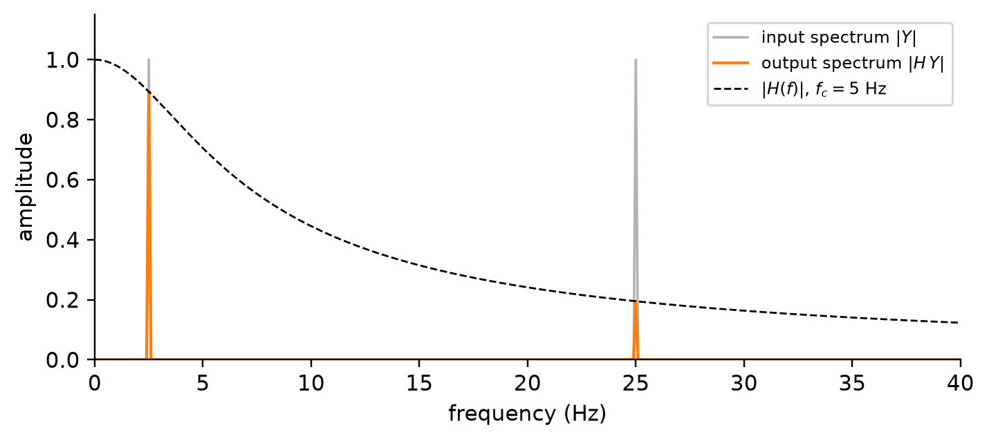
so that \(|H| = 1/\sqrt{1 + (f/f_c)^2}\) and \(\angle H = -\tan^{-1}(f/f_c)\). With \(C = 0.1\ \mu\mathrm{F}\), \(f_c \approx 50\) Hz, as in Lecture 5. With \(C = 1\ \mu\mathrm{F}\), \(f_c \approx 5\) Hz, and Figure 7.11 shows what Equation 7.23 then does to a structure with modes at 2.5 and 25 Hz: the first mode passes at 89% of its amplitude and lagging by 27°, the second arrives at 20% (−14 dB) — attenuated before it ever reaches the ADC, and, if nobody looked at the capacitor, silently absent from the spectrum. The lesson is not that filtering is bad; it is that a modal peak that is missing from a spectrum may be missing because of the chain, not the structure, and Equation 7.23 is how you check.
Figure 7.11: The convolution theorem applied to the sensor’s own filter. A synthetic vibration with modes at 2.5 Hz and 25 Hz (grey spectrum) passes through the ADXL335’s output RC filter with a 1 \(\mu\)F bandwidth capacitor (\(f_c \approx 5\) Hz; magnitude response dashed). The output spectrum (orange) is the product: the 2.5 Hz mode survives at 89%, the 25 Hz mode is cut to 20%.
The same equation runs backwards, and that is how sensors and structures are characterized. If you know the input as well as the output — a shaker table with an instrumented base, a calibrator driving a sensor — then \(H(f) = Y_{\mathrm{out}}(f)/Y_{\mathrm{in}}(f)\), frequency by frequency, is a measured transfer function: the sensor’s frequency response, or the structure’s, with its resonances standing up as peaks. Without an input channel one is left with the output spectrum alone, which mixes the structure’s \(|H|\) with whatever spectrum the excitation had; that is the situation in the case study that follows, and it is worth knowing what you are giving up.
CautionConcept Check: Two filters in cascade
A signal component passes through two first-order low-pass filters, each with its corner exactly at that component’s frequency. By how much is it attenuated, and what happens to its phase?
TipAnswer
Each filter contributes \(-3\) dB and \(-45°\) at its own corner. By Equation 7.24 the magnitudes multiply — \((1/\sqrt{2})^2 = 1/2\), that is \(-6\) dB — and the phases add, to \(-90°\). In decibels the attenuations simply add, \(-3 + (-3) = -6\); what one must not do is add the linear magnitudes or multiply the phases.
7.6 Case Study: Modal Frequency from Accelerometer Data
A two-story frame sits on a shaker table with eight accelerometers on its floors, and the first question a structural engineer asks of such a record is “what are the natural frequencies?” — the numbers that decide whether a design resonates with traffic, wind, or an earthquake. We apply the windowed FFT to the eight channels, read off the dominant peaks, and use the sensor layout to attribute each peak to translation or rotation of a story.
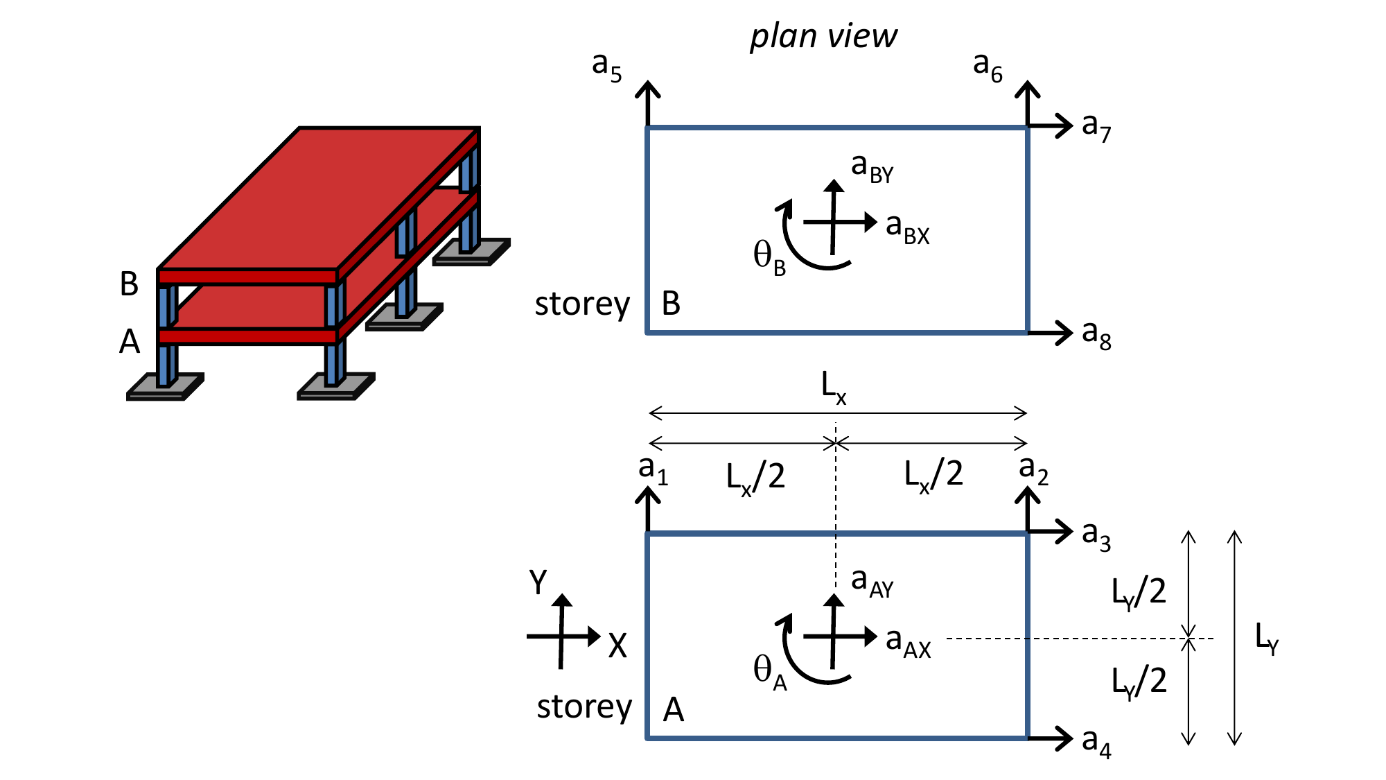
The data were collected by Matteo Pozzi and are shared here with permission. The record holds 25 s of response at \(f_s = 200\) Hz — 5000 samples on each of eight channels, \(a_1\) through \(a_8\) — from a two-story frame excited through its base. Figure 7.12 shows where the sensors sit: on each story, two accelerometers measure in the \(Y\) direction at the two ends of one edge and two measure in the \(X\) direction at the two ends of a perpendicular edge, so that each floor’s motion in its own plane — two translations and a rotation — is captured by four sensors. Only the response was recorded; there is no channel for the shaker’s own motion, so this is output-only analysis, with the limitation just described in Section 7.5.
Figure 7.12: The instrument layout: stories A (lower) and B (upper) of the frame, in plan view. Channels \(a_1\), \(a_2\) (\(a_5\), \(a_6\)) measure \(Y\)-acceleration at the two ends of one edge of story A (B); \(a_3\), \(a_4\) (\(a_7\), \(a_8\)) measure \(X\)-acceleration at the two ends of a perpendicular edge. Each story’s in-plane motion — \(a_X\), \(a_Y\), and the rotation \(\theta\) about the vertical — is recoverable from its four channels. Layout courtesy of Matteo Pozzi.
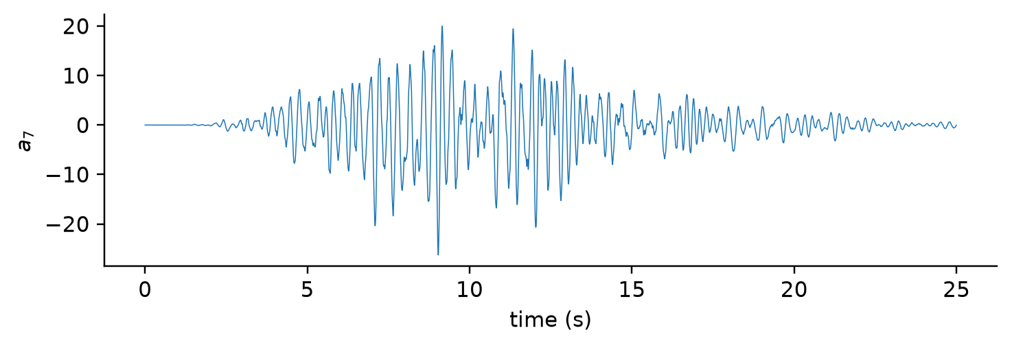
Look at the record before transforming it — always. Figure 7.13 shows channel \(a_7\): quiet for the first two seconds, a strong burst of motion through the middle of the record, and a decay. This is a transient, not a stationary signal, so there is no steady process whose average power we could estimate — the power spectral density of the optional callout in Section 7.4 would describe a process, not this event. What we want is the amplitude spectrum of Equation 7.17 of the whole record, Hann-windowed since the record certainly does not hold a whole number of cycles of anything, with the mean removed first. The full 25 s buys \(\delta f = 0.04\) Hz, resolution enough to separate peaks a few tenths of a hertz apart.
Figure 7.13: Channel \(a_7\) (story B, \(X\) direction) over the full 25 s record: a transient response to base excitation, with a quiet lead-in, a strong burst, and a decay. A record like this is analyzed with the windowed amplitude spectrum, not a stationary PSD.
The analysis is four lines, and they are worth reading rather than folding away: remove the mean, window, transform, scale.
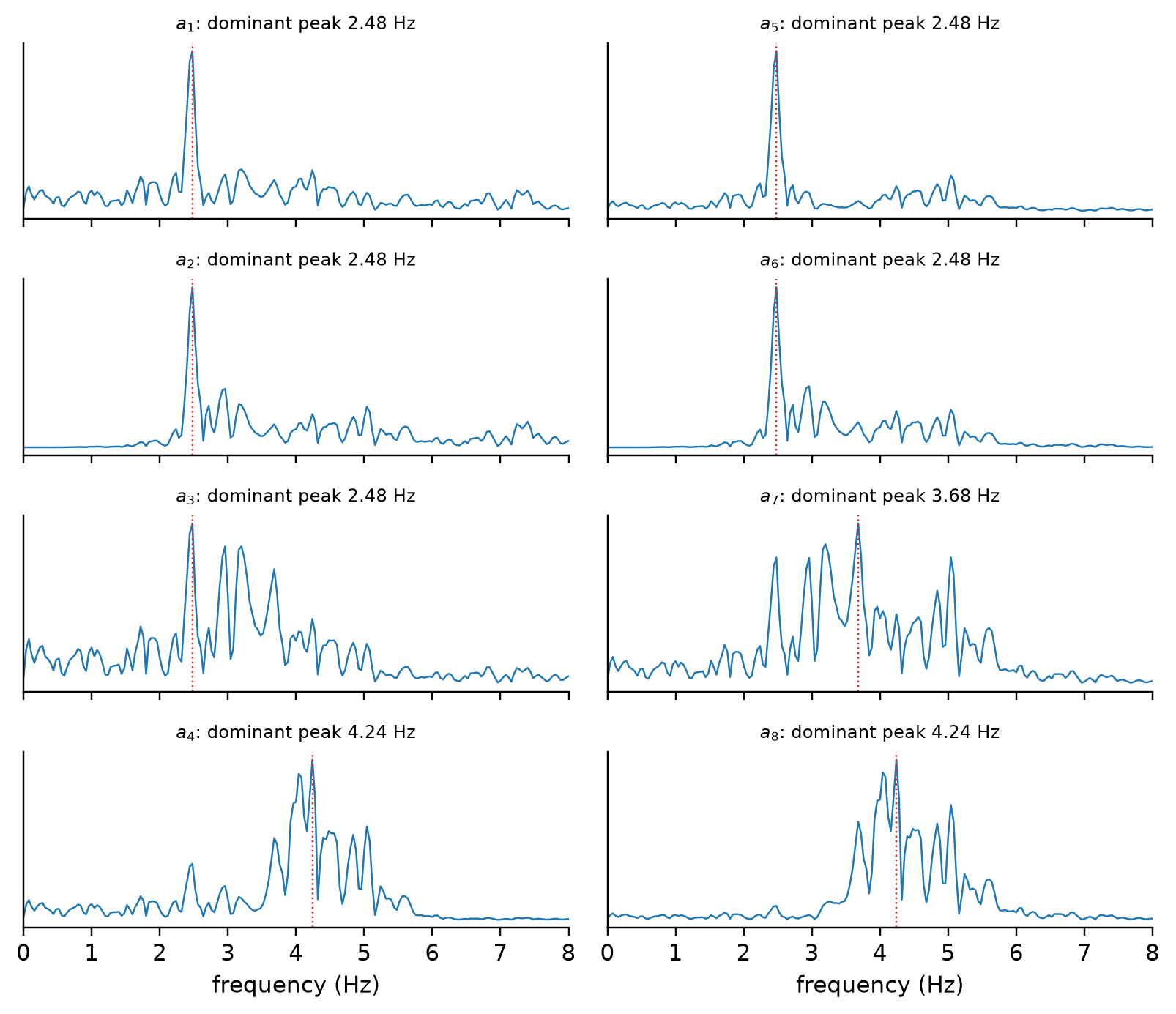
N_case =len(seis)w_case = np.hanning(N_case)f_case = np.fft.rfftfreq(N_case, 1/fs_case)def amp_spec(x): x = x - x.mean() # remove the dc componentreturn amp_spectrum(x, w_case) # window, transform, scale to amplitudespectra = np.column_stack([amp_spec(seis[:, c]) for c inrange(8)])dominant = f_case[np.argmax(spectra, axis=0)]fig, axs = plt.subplots(4, 2, figsize=(7.4, 6.4), sharex=True, sharey=False)for c, ax inenumerate(axs.T.flat): ax.plot(f_case, spectra[:, c], lw=0.8) ax.axvline(dominant[c], color="C3", lw=0.8, ls=":") ax.set_title(f"$a_{c +1}$: dominant peak {dominant[c]:.2f} Hz", fontsize=8) ax.set_xlim(0, 8); ax.set_yticks([])for ax in axs[-1]: ax.set_xlabel("frequency (Hz)")plt.tight_layout(); plt.show()
Figure 7.14: Hann-windowed amplitude spectra of all eight channels over the 25 s record (\(\delta f = 0.04\) Hz), 0–8 Hz, with the dominant peak of each channel marked. Every \(Y\) channel and \(a_3\) peak at 2.48 Hz; \(a_7\) peaks at 3.68 Hz; \(a_4\) and \(a_8\) peak at 4.24 Hz. The same handful of frequencies — 2.48, 2.96, 3.20, 3.68, 4.24, 5.04 Hz — recur across channels at different strengths.
Three things stand out in Figure 7.14. First, the dominant frequency depends on where you put the sensor: the \(Y\)-direction channels all peak at 2.48 Hz, the two \(X\) channels of story B at 3.68 Hz (\(a_7\)) and 4.24 Hz (\(a_8\)), and \(a_4\) at 4.24 Hz as well — a single accelerometer reports the mode it happens to sit on, which is why one never instruments a structure with one. Second, the same frequencies recur from channel to channel with different strengths — 2.48, 2.96, 3.20, 3.68, 4.24, and 5.04 Hz — which is the signature of modes: a natural frequency belongs to the whole structure, and each sensor sees it in proportion to how much that mode moves its location and direction. Third, the peaks are sharp and distinct because the record is long; the exercise at the end of the lecture shows what happens to them at a fifth and a twenty-fifth of the length.
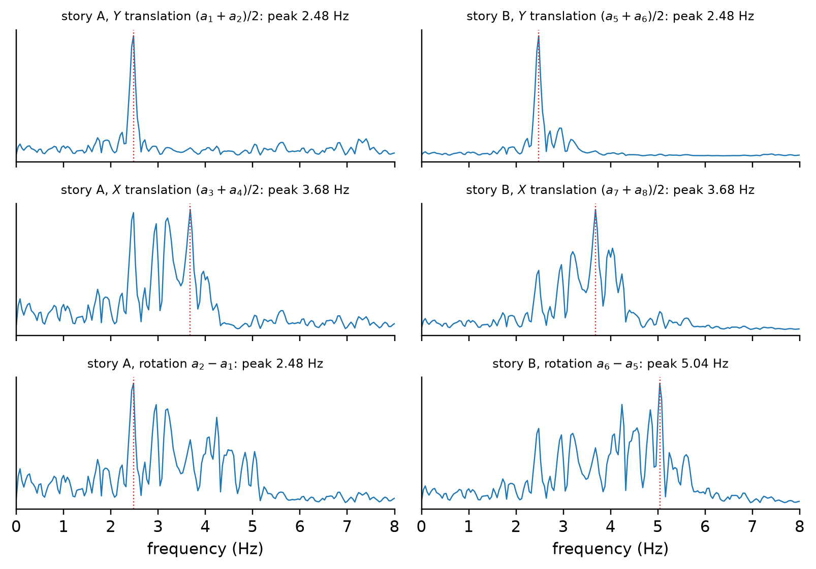
The layout in Figure 7.12 lets us go one step further and separate the motions before transforming. Rotation of a rigid floor about its vertical axis moves the two ends of an edge in opposite senses, translation moves them together; so on story A the average \((a_1 + a_2)/2\) is the \(Y\)-acceleration of the floor with the rotation cancelled, and the difference \(a_2 - a_1\) is the rotation with the translation cancelled — and likewise \((a_3 + a_4)/2\) and \(a_4 - a_3\) for the \(X\) direction and the same rotation. Figure 7.15 shows the spectra of these combinations. The \(Y\)-translation of each story is dominated by 2.48 Hz alone; the \(X\)-translation of story B peaks at 3.68 Hz; and the rotation of story B is dominated by 5.04 and 4.24 Hz, peaks that were minor in every raw \(Y\) channel. (That \(a_2 - a_1\) and \(a_4 - a_3\) have identical spectral shapes is a check that the floor is behaving as a rigid body: both are the same rotation, scaled by the edge lengths.) Which mode a peak belongs to has become a question the geometry can answer.
Figure 7.15: Spectra of channel combinations that isolate each story’s motions. Averaging the two sensors on an edge cancels rotation and leaves translation; differencing them cancels translation and leaves rotation. \(Y\)-translation of both stories is dominated by 2.48 Hz alone; \(X\)-translation of story B by 3.68 Hz; rotation of story B by 5.04 and 4.24 Hz, peaks the raw \(Y\) channels barely showed.
What we have not done is prove that every peak is a mode. Output-only spectra are the product of the structure’s response and the excitation’s spectrum (Equation 7.23), and a shaker with a strong component at some frequency would leave a peak there too; a recorded base channel would settle it by division. Nor have we extracted damping or mode shapes, which are the business of a structural dynamics course. What the FFT has delivered, in four lines of code, is the list of frequencies at which this structure prefers to move and a first assignment of each to a story and a direction — which is what a sensing engineer hands to the structural engineer, and what the next lecture teaches you to attach an uncertainty to.
TipActive Learning: Predict the grouping
Cover Figure 7.14 and look only at the layout in Figure 7.12. Which channels should share a dominant peak (same direction, same story)? Which pairs should show identical spectral shapes if the floors are rigid? Which combination of channels would you form to see the rotation of story A on its own? Write your predictions down, then uncover the figures and check each one.
7.7 Putting It All Together
The lecture opened with a summary that could not tell a signal from its shuffled copy and closed with a spectrum that names a building’s modes, and every step between was one more assumption made explicit about a finite record. The Fourier series decomposes a periodic signal into harmonics; the transform is its limit for signals that never repeat; the DFT is the transform we can compute, at the price of pretending the record repeats; windows pay that price gracefully; the PSD, if you took the optional detour, extends all of it to random signals; and the convolution theorem turns every LTI block in the chain — sensor, filter, structure — into a multiplication that can be read off a Bode plot. Each of the three questions of Section 7.2 now has its place in the spectrum: the mean is bin zero, the RMS is the square root of the area, and how the signal moves is the shape of the curve in between.
This is the last purely signal-side tool in the SENSORS third. Lecture 7 asks how much of what the spectrum shows is the structure and how much is the measurement — noise, quantization, and the uncertainty that every number in Figure 7.14 deserves to carry. After that the DATA third takes custody of the record, and the spectrum will reappear when time-series data need to be stored, compressed, and modeled.
7.8 Exercises
A pump’s output pressure is a full-wave-rectified 60 Hz sine, \(p(t) = |P_0 \sin 120\pi t|\).
State its period and fundamental frequency, and explain why its Fourier series contains only cosine terms.
Compute \(A_0\) in terms of \(P_0\).
A logger samples this pressure at 1 kS/s for 0.5 s; on which bins do the fundamental and its first two harmonics fall, and is there leakage?
TipSolution
\(|\sin 120\pi t|\) repeats every half cycle of the sine: the period is \(1/120\) s and the fundamental is 120 Hz — twice the supply frequency, which is why lamp flicker is at 120 Hz. The function is even about \(t = 0\), so all \(B_n = 0\) (Equation 7.7 with an odd integrand).
By Equation 7.7, \(A_0 = \frac{1}{T}\int_{-T/2}^{T/2} P_0|\sin 120\pi t|\,\mathrm{d}t = 2P_0/\pi \approx 0.637 P_0\): the mean of a rectified sine is \(2/\pi\) of its peak.
\(N = 500\) and \(\delta f = 2\) Hz, so 120, 240, and 360 Hz fall exactly on bins 60, 120, and 180: no leakage, because \(0.5\) s holds exactly 60 periods.
A 60 Hz hum is sampled at 400 Hz for 64 samples.
Which bin does it fall nearest, and is there leakage?
Find the shortest record length \(N\) for which there is none.
Would a Hann window help in case (a), and what would it cost?
TipSolution
\(\delta f = 400/64 = 6.25\) Hz and \(60/6.25 = 9.6\): the tone sits between bins 9 (56.25 Hz) and 10 (62.5 Hz), and the record holds 9.6 cycles, so it leaks into every bin.
One cycle of 60 Hz is \(400/60 = 6\tfrac{2}{3}\) samples, so the record holds a whole number of cycles when \(N\) is a multiple of 20 (three cycles): \(N = 20\), with \(\delta f = 20\) Hz and the tone exactly on bin 3.
Yes: the far skirt drops by an order of magnitude and the largest bin reads closer to the true amplitude after the factor-of-2 correction, at the cost of the peak spreading over two bins — which here is harmless, since there is only one tone to resolve.
(Optional; uses the power spectral density callout in Section 7.4.) From the PSD in the floor-vibration exercise there, compute the RMS acceleration in the 1–4 Hz band alone and in the 4–10 Hz band alone, and explain why the two do not add to the 1–10 Hz RMS.
TipSolution
Band variances are \(6 \times 10^{-4}\) and \(3 \times 10^{-4}\ (\mathrm{m/s^2})^2\), so the band RMS values are \(0.0245\) and \(0.0173\ \mathrm{m/s^2}\). Their sum, \(0.042\), exceeds the 1–10 Hz RMS of \(0.030\) because it is variances that add across disjoint bands (Equation 7.21), not RMS values: \(\sqrt{6 \times 10^{-4} + 3 \times 10^{-4}} = 0.030\).
A first-order low-pass filter with a 50 Hz corner precedes the ADC. A modal peak sits at 30 Hz.
By how much is its amplitude attenuated, in linear terms and in decibels, and how much phase does it acquire?
A second, identical filter is added in cascade; repeat.
You need the 30 Hz peak within 5% of its true amplitude with one filter; find the lowest corner frequency that achieves it.
TipSolution
\(|H| = 1/\sqrt{1 + (30/50)^2} = 0.857\), or \(-1.34\) dB, with a phase of \(-\tan^{-1}(0.6) = -31.0°\).
By Equation 7.24 the magnitudes multiply, \(0.857^2 = 0.735\) (\(-2.68\) dB, the decibels adding), and the phases add to \(-62.0°\).
\(1/\sqrt{1 + (30/f_c)^2} \geq 0.95\) requires \((30/f_c)^2 \leq 1/0.95^2 - 1 = 0.108\), so \(f_c \geq 30/0.329 \approx 91\) Hz.
Using channel \(a_7\) of the case-study data, compute the Hann-windowed amplitude spectrum of:
the full 25 s record;
the 5 s from \(t = 8\) s to 13 s;
the 1 s from \(t = 8\) s to 9 s.
Report \(\delta f\) and the dominant peak of each, and explain what became of the peaks at 2.96, 3.20, and 3.68 Hz.
TipSolution sketch
\(\delta f = 0.04\) Hz: peaks at 2.48, 2.96, 3.20, 3.68, and 5.04 Hz, dominant at 3.68 Hz.
\(\delta f = 0.2\) Hz, and the Hann window’s main lobe reaches two bins (0.4 Hz) to either side of each mode, wider than the gaps between 2.96, 3.20, and 3.68 Hz. The three stop producing peaks of their own: the dominant peak is at 3.2 Hz, 3.68 Hz survives only as a falling shoulder at 3.4–3.6 Hz, and 2.96 Hz blends into a broad plateau from 2.4 to 2.8 Hz. The next-largest peaks sit at 2.4, 4.0, and 5.0 Hz.
\(\delta f = 1\) Hz: everything between 2.5 and 3.7 Hz collapses into one hump at 3 Hz, and the dominant “peak” is a bin 1 Hz wide. Resolution is record length (Equation 7.16), and closely spaced modes need seconds of data, not samples.
Cooley, James W., and John W. Tukey. 1965. “An Algorithm for the Machine Calculation of Complex Fourier Series.”Mathematics of Computation 19 (90): 297–301. https://doi.org/10.2307/2003354.
Figliola, Richard S., and Donald E. Beasley. 2019. Theory and Design for Mechanical Measurements. 7th ed. Wiley.
Harris, Fredric J. 1978. “On the Use of Windows for Harmonic Analysis with the Discrete Fourier Transform.”Proceedings of the IEEE 66 (1): 51–83. https://doi.org/10.1109/PROC.1978.10837.
Lyons, Richard G. 2010. Understanding Digital Signal Processing. 3rd ed. Prentice Hall.
Oppenheim, Alan V., Alan S. Willsky, and S. Hamid Nawab. 1997. Signals and Systems. 2nd ed. Prentice Hall.
Welch, Peter D. 1967. “The Use of Fast Fourier Transform for the Estimation of Power Spectra: A Method Based on Time Averaging over Short, Modified Periodograms.”IEEE Transactions on Audio and Electroacoustics 15 (2): 70–73. https://doi.org/10.1109/TAU.1967.1161901.