9Lecture 08: Time-Series Data: Representation and Processing
9.1 Lecture Overview
NoteLearning Objectives
By the end of this lecture, students should be able to:
Represent time-series data unambiguously, handling timestamps, time zones, and irregular sampling
Decompose a time series into trend, seasonal, and residual components to reveal patterns in sensor data
Resample, interpolate, and align time series recorded at different rates or with gaps, using regression to estimate unobserved values
Detect and handle missing values and outliers in sensor data (e.g., using Chauvenet’s criterion), and articulate the assumptions each strategy makes
Explain what virtual sensors are and how they derive measurements from other sensors or models
Compute rolling statistics and apply simple smoothing filters to noisy measurements
Compare storage formats for time-series data (CSV, Parquet, purpose-built time-series databases) in terms of size, speed, and interoperability
Use pandas to carry out all of the above on real sensor data
NoteTopics Covered
What a sensor record contains, and single-table, multi-table, and synchronous layouts
Timestamps, time zones, and the three clocks in a sensor record
Noise: probability distributions, averaging, and sample statistics
Rolling statistics and smoothing filters
Missing values, duplicates, and outliers, including Chauvenet’s criterion and a robust alternative
Resampling, interpolation, and alignment across sampling rates
Decomposition by time scale, and into trend, seasonal, and residual components
Optional: STL and multiplicative decomposition
Virtual sensors, their noise, and the difference between measurement uncertainty and model error
Storage formats: CSV, Parquet, and time-series databases
9.1.1 Before You Begin
This lecture opens the DATA third and leans on three earlier ones: Lecture 5 for sampling and the meaning of \(x[n]\), Lecture 6 for why a record’s length and rate matter, and Lecture 7 for Type A and Type B uncertainty and for propagation through a function of several inputs. The probability and statistics this lecture needs (distributions, means and variances, and what averaging does to noise) are summarized where they are used. Most of the ideas are taught through interactive figures in the web version of these notes; the pandas operations that implement each idea are collected in short folded blocks labeled In pandas, as vocabulary to reach for rather than code to study.
To follow along on your own machine, save these files in a data/ folder next to your notebook, keeping the plaid/ subfolder, so that the paths in the code blocks work as written:
The shaker-table records of Section 9.8.2 are the one exception: they were shared with me for use in this course, not for public posting, so ask me or the TA for a copy.
9.2 From Signals to Records
Lectures 5 through 7 treated a measurement as \(x[n]\): a sample index, an implicit uniform spacing, and no wall clock anywhere in sight. The moment that record is written to a file, someone else has to be able to say exactly when each sample was taken, and this section establishes the three distinct pieces of timing information that make a record unambiguous.
Most of this lecture is built on one record. It comes from an Assignment 1 kit (the GL5528 divider and the HC-SR501 on an ESP32) left running in an office for two days, with the starter logger’s sample interval raised from 250 ms to one minute and a laptop capturing the serial stream; the laptop’s capture script writes each line to a file prefixed with the laptop’s own clock. The record, data/room_light_pir.csv, is simulated: a script, make_lecture08_data.py, generated it to behave like a real deployment, and because it is simulated, we know what really happened in the room and can check every repair against the truth. The first lines look like this:
A second file, data/outdoor_irradiance.csv, holds the global horizontal irradiance reported by a (likewise simulated) rooftop weather station over the same two days, one value every fifteen minutes.
9.2.1 What a Sensor Record Contains
A number in a file is useless until someone knows which sensor produced it, when, in what units, and how it was converted, and a network of sensors multiplies that bookkeeping by the number of sensors. A record is measurements plus timestamps plus metadata, and how those three are laid out in tables is a design decision with consequences that reach all the way to the databases of the next lectures.
A sensor network, whether the eight accelerometers on a laboratory frame, the strain and temperature sensors on the cables of a cable-stayed bridge, or a few hundred room kits across a campus, produces three kinds of data. The measurements are the values themselves. The timestamps say when each value was taken. The metadata say what each sensor is: its calibration (how its raw output converts to a physical quantity), its unit, and its position. Lose the timestamps and the measurements cannot be related to anything else; lose the metadata and they cannot even be interpreted.
When one sensor is sampled at a constant interval \(\Delta t\), its timestamps follow \[
t_i = t_0 + i\,\Delta t, \qquad i = 0, 1, 2, \ldots, N-1,
\tag{9.1}\] and its record is a time series: the sequence of values \(y_i\), where \(y_i\) is the \(i\)-th value of the time history, collected into a vector \(\mathbf{y}\) of measurements for that one sensor. The records of several sensors sampled together form a matrix \(\mathbf{M}\), one row per time and one column per sensor, so that each column of \(\mathbf{M}\) is one sensor’s \(\mathbf{y}\). This is the \(x[n]\) of Lectures 5 and 6 with the two facts they left implicit written down: when sample 0 was taken, and how far apart the samples are. From here on, a measurement is written \(y_i\).
The same data can be laid out in tables in more than one way. The single-table scheme (Table 9.1) has one row per measurement, carrying its time, its value, its sensor, and everything known about that sensor. It is complete and self-describing, but the calibration, unit, and position are repeated on every row of the same sensor. That repetition wastes space, and it invites inconsistency: correct a sensor’s calibration and every one of its rows must change, or the table contradicts itself.
Table 9.1: The single-table scheme: one row per measurement, with the sensor’s metadata repeated on every row. Times are UTC on Sunday 2 November 2025.
time (UTC)
value
sensor ID
calibration
unit
position
19:36:21Z
3600
1
raw code
ADC code
desk
19:36:21Z
1
2
raw state
0/1
ceiling
19:37:00Z
263.0
3
as reported
W/m²
roof
19:37:21Z
3602
1
raw code
ADC code
desk
19:37:21Z
0
2
raw state
0/1
ceiling
The multi-table scheme (Table 9.2) stores each fact once. The measurements table holds only the time, the value, and a sensor ID; a second table holds what is known about each sensor, one row per sensor; the ID links the two. Correcting a calibration now means changing one cell. This separation of facts into tables linked by identifiers is the founding idea of the relational databases of Lectures 9 through 11.
Table 9.2: The multi-table scheme: the same data as Table 9.1, with each sensor’s metadata stored once.
(a) Measurements
time (UTC)
value
sensor ID
19:36:21Z
3600
1
19:36:21Z
1
2
19:37:00Z
263.0
3
19:37:21Z
3602
1
19:37:21Z
0
2
(b) Sensors
sensor ID
calibration
unit
position
1
raw code
ADC code
desk
2
raw state
0/1
ceiling
3
as reported
W/m²
roof
When the whole network is read at the same moment, a third layout is natural: the synchronous form (Table 9.3), one row per scan and one column per sensor, all sharing one timestamp. It is the matrix \(\mathbf{M}\) with a column of times attached. The Assignment 1 logger writes this form, since the light and PIR readings of one sample share a line. It is compact, and it is the shape most analysis wants, but it works only when the sensors really are read together: the weather station, which reports every fifteen minutes at its own times, cannot share rows with the kit until someone decides how to align the two (Section 9.6).
Table 9.3: The synchronous form: one row per scan, one column per sensor. Times are UTC on Sunday 2 November 2025.
time (UTC)
sensor 1: light (ADC code)
sensor 2: PIR (0/1)
19:36:21Z
3600
1
19:37:21Z
3602
0
19:38:21Z
3603
1
With a record laid out, the work on it falls into a few kinds. Cleaning it: finding outliers, filling missing data, reducing noise. Describing it: identifying trends and cycles, extracting the features that matter. Using it: making inferences about the past and present, and predictions about the future. And combining the outcomes of many sensors into quantities none of them measures alone. This lecture covers cleaning, describing, and combining; extracting features, inference, and prediction are the business of the MODELS third of the course.
9.2.2 Three Clocks in One Record
An ESP32 wakes up believing it is January 1970, counts milliseconds since boot, and knows nothing whatsoever about Pittsburgh, and every one of those facts ends up in the log it writes. Sample index, device elapsed time, and wall-clock time answer different questions and fail in different ways, so a defensible record keeps all three instead of collapsing them into one column.
The sample index\(i\) is the row’s position in the file. It is what Lectures 5 and 6 called time, and it is the only clock that never lies about order of arrival, but it says nothing about spacing: a gap in the record is invisible to it.
The device elapsed time, time_ms, is the ESP32’s millis(): milliseconds since the chip last powered up. Its spacing is excellent. The starter logger fires a sample as soon as it notices that millis() has advanced by at least the interval since the last one, so in this record consecutive values differ by 60,000 or 60,001 ms, the extra millisecond appearing whenever the loop noticed a moment late. But it restarts at zero whenever the board does, it runs on the ESP32’s own crystal rather than on anybody’s official time, and it has no idea what day it is.
The wall-clock time, host_time, is the laptop’s clock, which is kept on official time over the network and therefore connects the record to the calendar, the weather, and the building’s schedule. It is written to the nearest second, it includes the few milliseconds the line spent in the USB serial link, and it stops whenever the laptop does.
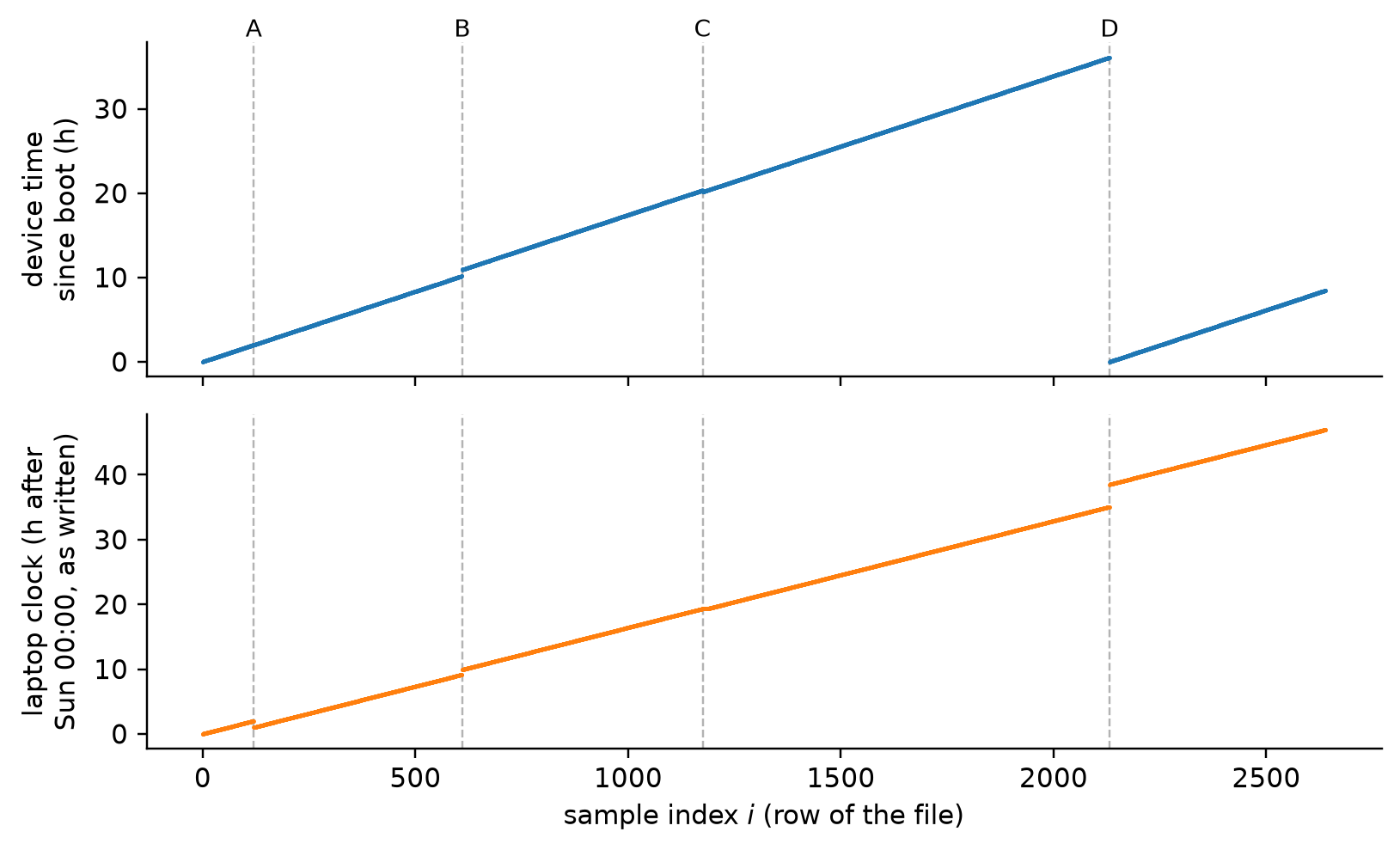
Reading the three side by side is the fastest way to find out what happened to a record. Figure 9.1 does it for the whole file, and each of the four events that break the record shows up with a different signature.
Figure 9.1: The same 2640 rows against their three clocks. Top: device elapsed time since boot, from time_ms. Bottom: the laptop’s clock exactly as written, read as naive local time. (A) daylight saving time ended, and only the laptop’s clock jumps back, by an hour; (B) the laptop slept, and both clocks jump forward together; (C) the capture script re-wrote twelve buffered lines, and only the device clock jumps back; (D) the kit lost power, and the device clock restarts at one minute while the laptop’s clock jumps three and a half hours ahead.
Table 9.4: How each of the four events looks on each clock.
Event
time_ms
laptop clock
What it means
(A) daylight saving ends
normal
jumps back 59 minutes
nothing happened in the room
(B) laptop sleeps
jumps 46 intervals
jumps 46 minutes
45 samples were taken and lost
(C) re-written lines
jumps back 11 intervals
+4 s
twelve rows are copies
(D) power lost
restarts at 60,000
jumps 3 h 28 min
about 207 samples were never taken
The table is the argument for keeping all three. The sleep and the power loss both open a gap in the laptop’s clock, but only the device clock can tell them apart, and only for the sleep can it say exactly how many samples went missing: time_ms advanced by 46 intervals, so 45 samples were taken and never written down. The re-written lines would pass unnoticed by anyone reading only the laptop’s clock, and the daylight-saving jump would look like data loss to anyone reading only that clock too. The two clocks also drift apart slowly: in this record the device clock gains 3.7 s on the laptop’s over the 36 hours before the power cut, a reminder that no clock is the truth, only a clock you have chosen to trust.
9.2.3 Time Zones, UTC, and Daylight Saving
On the first Sunday in November a building’s local clock reads 01:30 twice, and the overnight mean computed from that log is quietly wrong in a way nobody can see by looking at the number. A timestamp without an explicit offset is not a timestamp, and storing UTC while converting to local time only for display makes both daylight-saving failures, the repeated hour and the missing one, impossible to hit.
At 02:00 Eastern Daylight Time (UTC−4) on Sunday 2 November 2025, clocks in Pittsburgh went back to 01:00 Eastern Standard Time (UTC−5). The laptop’s clock did what it was told, so rows 60 through 119 carry the stamps 01:00:22 through 01:59:22, and rows 120 through 179 carry the same stamps again, an hour later. Read naively, the file claims that 120 samples were taken in one hour, and anything that groups by hour will double-count it; sort the file by that column and the two passes interleave. The day itself was 25 hours long, which matters to anyone computing a daily total. The mirror-image failure happens in spring: on Sunday 8 March 2026, local times from 02:00 to 02:59 never existed, and a naive log simply has no such rows, which reads like an hour of missing data.
The fix is to attach the offset while the information needed to choose it still exists. Here it does: the rows are in order, so the first pass through the repeated hour must be EDT and the second EST. The weather station’s file shows what a finished record should look like: 2025-11-02T04:07:00Z, an ISO 8601 timestamp in UTC (the trailing Z), which means the same instant in every time zone and needs no rule to interpret. Store that; convert to local time only when a human needs to read it.
In pandas
import pandas as pdroom = pd.read_csv("data/room_light_pir.csv")naive = pd.to_datetime(room["host_time"]) # no offset yetlocal = naive.dt.tz_localize("America/New_York", ambiguous="infer") # order picks EDT or ESTutc = local.dt.tz_convert("UTC") # store this...room["time_utc"] = utc.dt.strftime("%Y-%m-%dT%H:%M:%SZ") # ...like this
ambiguous="infer" works only because the rows are in order; if they were not, pandas raises an error rather than guessing, which is the right behavior. For the spring gap the corresponding argument is nonexistent=.
9.2.4 Irregular Sampling
The logger asks for one sample a minute, and a quick look at the file suggests it got one, but “one sample a minute” is a claim about the device’s intent, not about what landed in the file. The gap between nominal and achieved sampling is itself a measurement worth making, because every method in the rest of this lecture assumes a spacing you have not yet checked.
The check is a tally of the differences between consecutive timestamps, how many times each spacing occurs. On the device clock, 2636 of the 2639 differences are 60,000 or 60,001 ms and the other three are the events B, C, and D; on the laptop’s clock, 2575 differences are 60 s, 48 are 59 or 61 s (a second’s rounding plus a few milliseconds of serial delay), eleven are zero (the re-written lines), and the remaining handful mark the events, including one of −3540 s (the clock going back). Neither clock is irregular in the everyday sense, yet the record is: it has two holes, and a method that assumes one row per minute will slide every sample after the first hole to the wrong time.
Some sensors are irregular by design. A PIR sensor, a door contact, or a thermostat that reports only when its reading changes produces an event log, not a sampled signal, and for those “the sampling rate” is not defined at all; what matters is when each event happened and how long the record is known to be complete. Such a record is summarized by counting events, or adding up how long a state lasted, over fixed intervals, and it is plotted against its actual timestamps, never against the row number.
In pandas
import pandas as pdroom = pd.read_csv("data/room_light_pir.csv")room["time_ms"].diff().value_counts() # tally of device stepspd.to_datetime(room["host_time"]).diff().value_counts() # and laptop steps
9.3 Noise and Its Statistics
Every operation in the rest of this lecture, from smoothing to outlier rejection to combining sensors, rests on a judgment about which part of a record is the quantity being measured and which part is noise. This section, which is the groundwork for the smoothing, outlier, and virtual-sensor methods that follow, gives that judgment a model and a vocabulary: a measurement as a quantity plus noise, the noise as a random variable with a distribution, and the statistics that describe the distribution and that can be estimated from the record itself.
9.3.1 Signal and Noise
A reading of 494 from the light sensor at three in the morning is not the light level; it is the light level plus whatever the circuit, the converter, and the environment added on the way. Writing that down as a model, and deciding which part is which, is the first step of every cleaning method in this lecture.
The model is additive: \[
y_i = q_i + n_i,
\tag{9.2}\] where \(y_i\) is the \(i\)-th measurement, \(q_i\) is the physical quantity at that moment, and \(n_i\) is the noise: a distortion affecting the signal, an unwanted component to be removed where it can be. Noise here is meant broadly, as anything in the record that is not the quantity of interest.
Two kinds of evidence identify noise in practice.
Correlation with a known noise source. If the source of a disturbance can itself be measured, whatever in the record moves with that reference is noise. Mains interference (Lecture 5) gives itself away by following the 60 Hz of the supply; the temperature sensitivity of a strain gauge gives itself away by following a thermometer mounted beside it.
Frequency content. When the physical quantity varies slowly, fast-varying components are noise: room light and air temperature change over minutes, so minute-to-minute jitter is noise, and smoothing (Section 9.4) removes it. When the quantity varies fast, slow-varying components are noise: an accelerometer on a vibrating floor measures oscillations of a few hertz, so a slow drift or offset in its output is noise, and the high-pass filtering of Lecture 5 removes it. The spectrum of Lecture 6 is the tool for telling the two apart.
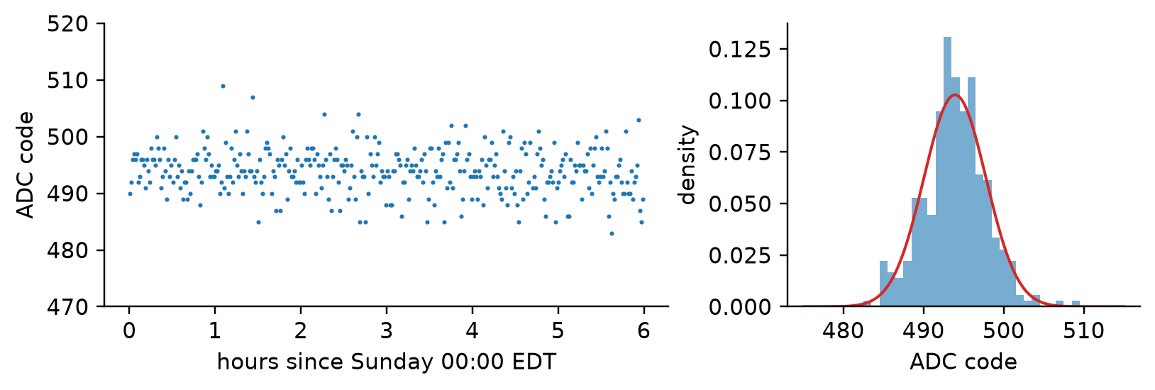
The cleanest view of the kit’s noise in the two-day record is the first six hours of Sunday, from midnight to 05:00 local time (six hours, not five, because of the repeated hour of Section 9.2.3). The room is dark and the light is constant, so \(q_i\) does not change and every wiggle in \(y_i\) is \(n_i\). Leaving out the one glitch in that stretch (a single corrupted reading, row 281, of the kind Section 9.5 deals with), the 359 readings average 493.9 codes and scatter about that value with a standard deviation of 3.9 codes (Figure 9.2). The rest of this section explains exactly what those two numbers are.
Figure 9.2: The kit’s noise, seen where the light is constant: the first six hours of Sunday, one glitch (circled) left out. Left: the readings in time order. Right: their histogram, scaled so that the bars’ total area is one, with the normal distribution of the same mean and standard deviation drawn over it.
9.3.2 Describing Noise with a Probability Distribution
Noise cannot be predicted reading by reading, but it can be described: how often it takes each size, where it is centered, how far it strays. That description is a probability distribution, and two numbers, its mean and its variance, summarize most of what matters about it.
A continuous random variable \(Y\) is described by its probability density function (PDF), \[
p(y) \triangleq \lim_{\Delta y \to 0} \frac{\Pr\left[Y \in (y, y + \Delta y)\right]}{\Delta y},
\tag{9.3}\] the probability that \(Y\) lands in a small interval near \(y\), per unit width of the interval. It is non-negative, \(p(y) \ge 0\), and normalized, \(\int_{-\infty}^{\infty} p(y)\, dy = 1\), because \(Y\) must land somewhere. Following common engineering usage, from here on the same lowercase letter stands for a random quantity and for its values, so that \(\mathbb{E}[y]\) below means the expected value of the random reading \(y\). A histogram of many samples, scaled so that its bars’ areas add up to one, approximates \(p(y)\); that is how a PDF shows up in data, as on the right of Figure 9.2.
Four numbers summarize a distribution:
the mean, or expected value, \(\mu \triangleq \mathbb{E}[y] = \int y\, p(y)\, dy\), which says where the distribution sits;
the variance, the second moment about the mean, \(\sigma^2 \triangleq \mathbb{V}[y] = \mathbb{E}\left[(y - \mu)^2\right]\), which says how far it strays;
the standard deviation\(\sigma = \sqrt{\sigma^2}\), the same spread in the units of \(y\); and
the coefficient of variation\(\delta \triangleq \sigma / |\mu|\), the spread relative to the level, which is dimensionless and useful for comparing sensors that read on different scales. For the night readings it is \(3.9/493.9 = 0.8\%\). It is meaningful only when zero on the measurement scale means “none” and \(\mu\) is not near zero: a temperature in degrees Celsius has no meaningful coefficient of variation.
The distribution met most often is the normal (or Gaussian) distribution, \[
\mathcal{N}(y; \mu, \sigma^2) \triangleq \frac{1}{\sqrt{2\pi\sigma^2}} \exp\left[-\frac{(y - \mu)^2}{2\sigma^2}\right],
\tag{9.4}\] which is positive everywhere and integrates to one, and whose two parameters are exactly its mean and variance: if \(p(y) = \mathcal{N}(y; \mu, \sigma^2)\), then \(\mathbb{E}[y] = \mu\) and \(\mathbb{V}[y] = \sigma^2\). It is symmetric about \(\mu\), so its mean, mode, and median coincide at \(\mu\); \(\mu\) sets its position and \(\sigma^2\) its width, the uncertainty. A normal variable falls within one standard deviation of its mean 68.3% of the time (34.1% on each side), within two 95.4% of the time (13.6% more on each side), and within three 99.7% of the time (2.1% more on each side), leaving 0.1% beyond three standard deviations on each side. The night readings fall within one, two, and three of their standard deviations 65%, 94%, and 99% of the time, close enough to the normal proportions that the normal model describes this sensor’s noise well. Measuring a deviation in standard deviations, \(z = (y - \mu)/\sigma\), turns any normal variable into the standard normal, with mean 0 and variance 1, whose cumulative distribution function \(\Phi(z) = \Pr[Z \le z]\) is tabulated in every statistics text and computed by every statistics library.
The standard model for sensor noise combines these ideas. Each \(n_i\) in Equation 9.2 is normal with zero mean, \(n_i \sim \mathcal{N}(0, \sigma^2)\) for every \(i\), and the \(n_i\) are independent of one another, \(n_i \perp n_j\) for \(i \ne j\). Zero mean says the noise does not push the readings one way on average (a push one way would be a systematic error, the subject of calibration in Lecture 7); independence says that one reading’s noise tells you nothing about the next one’s. Noise with these properties is called white noise, by analogy with white light: independence from sample to sample makes its spectrum flat, with equal power at every frequency.
In pandas
import pandas as pdroom = pd.read_csv("data/room_light_pir.csv")night = room["adc_code"].iloc[:360].drop(index=281) # 6 h; row 281 glitchnight.mean() # sample meannight.std() # standard deviation, dividing by N - 1night.std() / night.mean() # coefficient of variation
9.3.3 Averaging Reduces Noise
If one reading of the night-time light is uncertain by 3.9 codes, a hundred readings of the same unchanging light should pin it down better: averaging is the oldest noise-reduction method there is. How much better follows from the white-noise model in a few lines, and both the answer and the conditions attached to it underlie every smoothing method in Section 9.4.
Suppose the quantity is constant, \(q_i = L\) (the length \(L\) of a table measured over and over, or the light in a dark room), so that each reading is \(y_i = L + n_i\) with white noise of variance \(\sigma^2\): then \(\mathbb{E}[y_i] = L\) and \(\mathbb{V}[y_i] = \sigma^2\). The arithmetic average of \(N\) readings is \[
\bar{y} = \frac{1}{N} \sum_{i=1}^{N} y_i.
\tag{9.5}\] Its expected value is \(\mathbb{E}[\bar{y}] = \frac{1}{N}\sum_i \mathbb{E}[y_i] = L\): averaging does not move the answer, so the average is an unbiased estimate of \(L\). Its variance is where the gain lies. For two readings, \[
\begin{aligned}
\mathbb{V}[\bar{y}] &= \mathbb{E}\left[\left(\tfrac{1}{2} y_1 + \tfrac{1}{2} y_2 - L\right)^2\right]
= \tfrac{1}{4}\, \mathbb{E}\left[\left\{(y_1 - L) + (y_2 - L)\right\}^2\right] \\
&= \tfrac{1}{4}\, \mathbb{E}\left[(y_1 - L)^2\right] + \tfrac{1}{4}\, \mathbb{E}\left[(y_2 - L)^2\right] + \tfrac{1}{2}\, \mathbb{E}\left[(y_1 - L)(y_2 - L)\right]
= \tfrac{1}{4}\sigma^2 + \tfrac{1}{4}\sigma^2 + 0 = \frac{\sigma^2}{2},
\end{aligned}
\tag{9.6}\] where the cross term vanishes because \(\mathbb{E}[(y_1 - L)(y_2 - L)] = \mathbb{E}[n_1 n_2] = 0\) for uncorrelated noise. The same steps work for \(N\) readings: squaring a sum of \(N\) deviations gives \(N\) squared terms, each contributing \(\sigma^2\), and \(N(N-1)\) cross terms, each zero, so \[
\mathbb{V}[\bar{y}] = \frac{N \sigma^2}{N^2} = \frac{\sigma^2}{N}, \qquad \operatorname{std}[\bar{y}] = \frac{\sigma}{\sqrt{N}}.
\tag{9.7}\] The argument never used the fact that the weights were all \(1/N\), and it did not need the readings to share one variance. For any weights \(\alpha_k\) and readings \(y_k\) with independent noise of variances \(\sigma_k^2\), the same expansion gives \[
\mathbb{V}\left[\sum_k \alpha_k y_k\right] = \sum_k \alpha_k^2 \sigma_k^2,
\tag{9.8}\] of which Equation 9.7 is the special case \(\alpha_k = 1/N\), \(\sigma_k = \sigma\). This general form returns in Section 9.8.1.
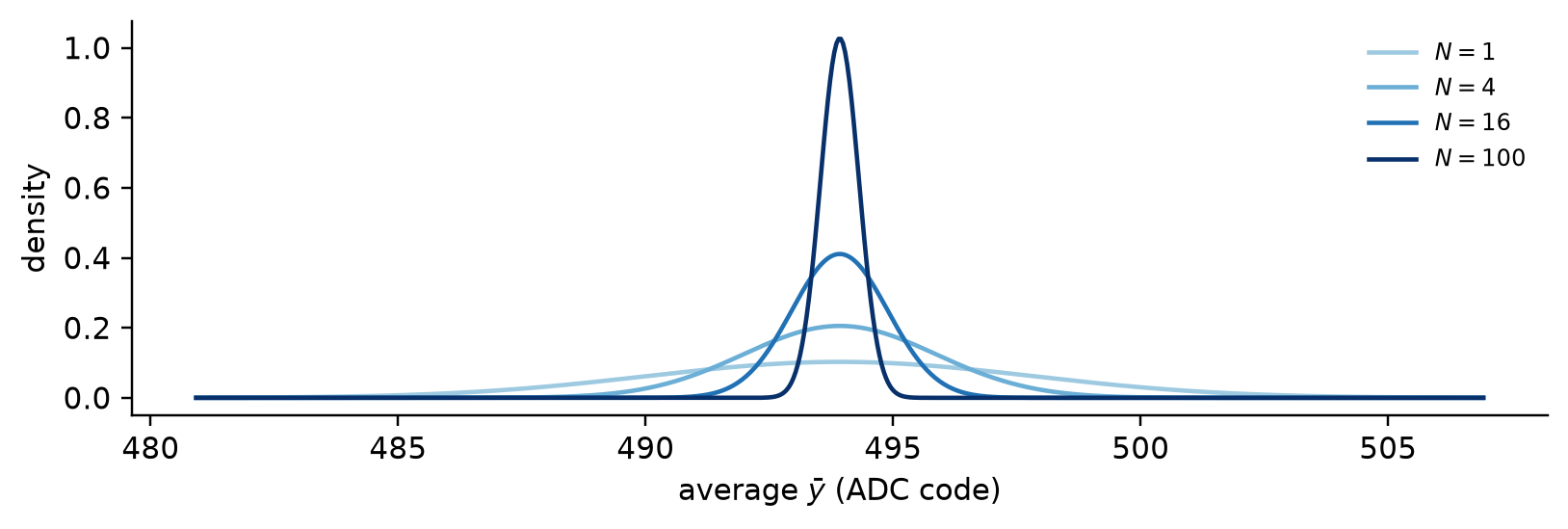
The square root is the practical lesson. The noise of an average shrinks with the square root of the number of readings, so halving it takes four times as many; averaging 16 night readings brings the kit’s 3.9 codes down to about 1 code (Figure 9.3). The conditions matter as much as the result. The noise must be uncorrelated: mains hum, which is the same in consecutive readings, averages away far more slowly. The quantity must be constant while the readings are taken: average across dawn and the average describes no moment of it. And only random error shrinks: a systematic error is the same in every reading and survives any amount of averaging, which is why Lecture 7 needed calibration as well.
Figure 9.3: The distribution of the average of \(N\) night-time readings, from the white-noise model with the kit’s \(\sigma = 3.9\) codes. Every curve is centered on the true level (the average is unbiased), and its width shrinks as \(\sigma/\sqrt{N}\).
9.3.4 Estimating the Mean and Variance from Samples
The mean \(\mu\) and variance \(\sigma^2\) belong to the distribution, which nobody gets to see; what we have is \(N\) readings. The sample mean and sample variance estimate them from the readings, and because the estimates are computed from random readings they are random too, closer to the truth the more readings they use.
The sample mean estimates \(\mu\) (the symbol \(\cong\) reads “is estimated by”): \[
\mu \cong \bar{y} \triangleq \frac{1}{N} \sum_{k=1}^{N} y_k .
\tag{9.9}\] For the variance, if \(\mu\) were known the natural estimate would be the average squared deviation from it, \(\frac{1}{N}\sum_k (y_k - \mu)^2\). It is not known, and replacing it by \(\bar{y}\) requires one change, dividing by \(N - 1\) instead of \(N\): \[
\sigma^2 \cong s^2 = \frac{1}{N - 1} \sum_{k=1}^{N} (y_k - \bar{y})^2 .
\tag{9.10}\] The reason is that \(\bar{y}\) is computed from the same readings, and it is the value that makes the sum of squared deviations as small as possible, so the readings sit closer to \(\bar{y}\) than to the true \(\mu\) and dividing by \(N\) would underestimate \(\sigma^2\) on average. Dividing by \(N - 1\) corrects the bias exactly, \(\mathbb{E}[s^2] = \sigma^2\); one says that one degree of freedom was spent on estimating the mean. For the 359 night readings the difference is invisible (3.883 against 3.878 codes); for four readings it changes \(s\) by 15%.
The widget below draws readings one at a time from a known distribution, a table of true length \(L = 5\) measured with noise of \(\sigma = 1\), and shows how the estimates settle as \(N\) grows. The true \(\mu \pm \sigma\) are the blue lines; the estimates \(\bar{y} \pm s\) from the first \(N\) readings are the red ones.
viewof nSamp = Inputs.range([2,200], {value:4,step:1,label:"number of readings N"})
sampPlot = {const y = sampleSeq.slice(0, nSamp), N = y.length;const m = d3.mean(y), s =Math.sqrt(d3.sum(y.map(v => (v - m) **2)) / (N -1));const pts = y.map((v, k) => ({k: k +1,y: v}));const p = Plot.plot({width:Math.min(760, width),height:260,marginLeft:45,x: {label:"reading k",domain: [0,200]},y: {label:"reading y",domain: [1.5,8.5]},marks: [ Plot.ruleY([4,5,6], {stroke:"#1f77b4",strokeWidth:1}), Plot.ruleY([m - s, m, m + s], {stroke:"#d62728",strokeDasharray:"5,3"}), Plot.line(pts, {x:"k",y:"y",stroke:"#999",strokeWidth:0.7}), Plot.dot(pts, {x:"k",y:"y",r:2,fill:"black"}), ], });const note =html`<div style="font-family:sans-serif;font-size:0.9em;margin-top:0.3em"> N = ${N}: estimates ȳ = ${m.toFixed(3)}, s = ${s.toFixed(3)} (true μ = 5, σ = 1)</div>`;returnhtml`<div>${p}${note}</div>`;}
9.4 Rolling Statistics and Smoothing
Two days of minute data is too noisy to show what you care about and too long to read line by line, and collapsing it to a daily mean throws away the timing that made it a time series in the first place. Rolling mean, median, and standard deviation summarize a signal while preserving time, and the exponentially weighted moving average is the same idea with an infinite window that fades rather than a finite one that ends.
A rolling statistic computes a summary over a window of \(w\) consecutive samples and assigns it to one of them. With a trailing window, the value at sample \(i\) summarizes samples \(i-w+1\) through \(i\), so the rolling mean is \[
r_i = \frac{1}{w} \sum_{k=0}^{w-1} y_{i-k},
\tag{9.11}\] and with a centered window of odd width \(w = 2\ell+1\) it summarizes samples \(i-\ell\) through \(i+\ell\). The rolling median and the rolling standard deviation replace the mean with those statistics, computed over the same window.
A rolling mean smooths for exactly the reason of Section 9.3.3. Where the quantity barely changes within the window, the rolling mean is an average of \(w\) noisy readings of the same value, so its noise is \(\sigma/\sqrt{w}\): an eleven-sample window cuts the kit’s night-time scatter from 3.9 codes to about 1.2. Where the quantity does change within the window, the same average blurs the change, and that is the price of smoothing.
The exponentially weighted moving average (EWMA) weighs every past sample, with weights that shrink geometrically into the past: \[
e_i = \lambda\, y_i + (1-\lambda)\, e_{i-1}, \qquad 0 < \lambda \le 1,
\tag{9.12}\] where the smoothing factor\(\lambda\) sets how fast old readings are forgotten: unrolled, Equation 9.12 gives the reading \(k\) samples back the weight \(\lambda(1-\lambda)^k\). It needs only its own previous output to compute the next one, which is why it is the smoother of choice on a microcontroller.
A useful way to compare smoothers is their mean delay: the average of the lags \(k\) of the readings they combine, each weighted by its weight. A trailing mean gives weight \(1/w\) to lags \(0\) through \(w-1\), so its mean delay is \((w-1)/2\) samples, about half a window. The EWMA’s weights give a mean delay of \(\sum_{k \ge 0} k\,\lambda(1-\lambda)^k = (1-\lambda)/\lambda\) samples. pandas parameterizes the EWMA by a span\(w\), with \(\lambda = 2/(w+1)\) (the library calls \(\lambda\)alpha), and the choice is not arbitrary: it makes \((1-\lambda)/\lambda = (w-1)/2\), the same mean delay as a trailing mean of width \(w\).
Two choices decide what a smoother does to a record. The window length trades noise for detail: a long window averages away the sensor’s scatter, and also any real event shorter than itself. The position of the window trades delay for availability: a centered window adds no delay but needs samples from the future, so a real-time system, which has only the past, must use a trailing window and accept its mean delay of about half a window.
The median is not just another average. A rolling mean is dragged by a single wild value; a rolling median ignores it as long as fewer than half the readings in the window are wild. Try both in the widget below, and watch what each does to the five single-sample glitches that the simulation inserted into the record.1
rollPlot = {const rows =transpose(rollRows), x = rows.map(r => r.code), n = x.length, w = roll.w;const lo = i => roll.pos==="centered"?Math.max(0, i - (w -1) /2) :Math.max(0, i - w +1);const hi = i => roll.pos==="centered"?Math.min(n -1, i + (w -1) /2) : i;const med = a => { const s =Float64Array.from(a).sort(), m = s.length>>1;return s.length%2? s[m] : (s[m -1] + s[m]) /2; };let y;if (roll.stat==="EWMA") {const al =2/ (w +1); y =newArray(n); y[0] = x[0];for (let i =1; i < n; i++) y[i] = al * x[i] + (1- al) * y[i -1]; } else { y = x.map((_, i) => { const s = x.slice(lo(i),hi(i) +1);return roll.stat==="mean"? d3.mean(s) :med(s); }); }const line = rows.map((r, i) => ({h: r.h,y: y[i]}));return Plot.plot({width:Math.min(760, width),height:280,marginLeft:50,x: {label:"hours since Sunday 00:00 EDT",domain: [0,48],ticks: d3.range(0,49,6)},y: {label:"ADC code",domain: [0,5100]},marks: [ Plot.dot(rows, {x:"h",y:"code",r:1,fill:"#9ecae1"}), Plot.line(line, {x:"h",y:"y",stroke:"#d62728",strokeWidth:1.2}), ], });}
In pandas
import pandas as pdy = pd.read_csv("data/room_light_pir.csv")["adc_code"]y.rolling(11, center=True).mean() # centered: needs the futurey.rolling(11).median() # trailing: all a live system hasy.rolling(11, center=True).std()y.ewm(span=11, adjust=False).mean() # lambda = 2/(span + 1)
9.5 Gaps, Duplicates, and Outliers
Ask for the mean light level in a room over two days and you get a number; nothing in that number reveals that the sensor was offline for three and a half hours, reported zero for forty minutes, and was counted twice for twelve. Detecting missing data, duplicates, and outliers is the easy half; the hard half is that every repair encodes an assumption about what happened while you were not looking, and this section makes each assumption say its name.
TipActive Learning: Six things wrong with this log
The nineteen lines below come from six places in the two-day record, with their line numbers in the file. Take three minutes, without a computer, and find six different problems. For each one, say what probably happened and whether any rows should be removed.
Lines 119 to 122: the laptop’s clock goes from 01:59 back to 01:00 while time_ms keeps counting (daylight saving ended; no rows to remove). Lines 611 and 612: both clocks jump 46 minutes (the laptop slept; 45 samples lost). Line 980: a code of 5012 on a 12-bit converter, whose largest code is 4095 (a corrupted line; remove or flag). Lines 1177 onward: time_ms goes backwards while the laptop’s clock moves forward (re-written copies; remove). Line 1904 onward: a code of exactly 0 at seven in the morning, repeated (a sensor lead came loose; the values are not light measurements). Lines 2133 and 2134: time_ms restarts at 60,000 and the laptop’s clock jumps three and a half hours (the kit lost power).
Each of these has a mechanical test, and the tests are worth writing down because they are cheap and they catch most of what goes wrong in a sensor record:
Range. A value the instrument cannot produce is wrong: a code above 4095, a negative relative humidity, a PIR state of 2.
Order and duplication. A key that should increase (time_ms within one boot) and goes backwards marks rows that are out of order or repeated.
Gaps. A spacing much larger than nominal marks missing samples; the device clock says how many.
Runs. A value repeated exactly, far longer than noise allows, marks a stuck sensor or a disconnected lead. A light sensor with four codes of noise does not read the same code forty times in a row.
In pandas
import pandas as pdroom = pd.read_csv("data/room_light_pir.csv")bad_range =~room["adc_code"].between(0, 4095) # rangecopies = room.duplicated(subset=["time_ms", "adc_code", "pir_state"])step = room["time_ms"].diff()gap_after = step >1.5*60000# gaps: spacing well over nominalreboot = step <-1e6# device clock restartedrun_id = (room["adc_code"] != room["adc_code"].shift()).cumsum()run_len = room.groupby(run_id)["adc_code"].transform("size")stuck = run_len >=10# same code ten or more timesroom["flag"] = bad_range | copies | stuck # flag, don't delete
A re-written copy repeats its original’s device time and readings, and only its laptop stamp differs, so it is found by looking for rows whose time_ms, adc_code, and pir_state all repeat an earlier row; the flag column keeps the evidence without destroying the rows.
Detection is the part that can be automated. Deciding what to do next is not, because each option is a claim about the missing or suspect values:
Table 9.5: Repair strategies for missing or suspect values, and what each one assumes.
Strategy
The claim it makes
Delete the rows
The values are missing for reasons unrelated to what they would have been.
Keep and flag
Whoever uses the data will read the flags.
Fill with zero
Nothing was there. For a sensor, this is almost never true.
Carry the last value forward
Nothing changed while we were not looking.
Interpolate
The quantity changed smoothly between the neighbours (Section 9.6).
Deleting looks like the neutral choice, and it is the one that most often is not. The kit lost power on Monday from 11:04 to 14:32, when the room was lit throughout and, apart from lunch, occupied; delete those hours and the record’s mean light level falls, because the rows that are left are disproportionately night. The widget below lets you make each decision and see what it does to a single summary number, the mean code over the two days, compared with what a perfect logger would have recorded.
viewof rep = Inputs.form({dup: Inputs.radio(["keep","delete"], {value:"keep",label:"re-written copies"}),oor: Inputs.radio(["keep","delete"], {value:"keep",label:"code 5012"}),stuck: Inputs.radio(["keep","delete"], {value:"keep",label:"stuck at zero"}),gaps: Inputs.radio(["leave out","fill with zero","carry last value"], {value:"leave out",label:"missing samples"}),})
repPlot = {const rows =transpose(roomRows);const drop = {1: rep.dup==="delete",2: rep.oor==="delete",3: rep.stuck==="delete"};const kept = rows.filter(r =>!drop[r.flag]);let sum = d3.sum(kept, r => r.code), n = kept.length;const g = gapInfo;if (rep.gaps==="fill with zero") n += g.sleepMissing+ g.outageMissing;if (rep.gaps==="carry last value") { sum += g.sleepMissing* g.sleepBefore+ g.outageMissing* g.outageBefore; n += g.sleepMissing+ g.outageMissing; }const mean = sum / n, err = mean - g.trueMean;const p = Plot.plot({width:Math.min(760, width),height:260,marginLeft:50,x: {label:"hours since Sunday 00:00 EDT",domain: [0,48],ticks: d3.range(0,49,6)},y: {label:"ADC code",domain: [0,5100]},marks: [ Plot.dot(rows.filter(r => drop[r.flag]), {x:"h",y:"code",r:1.6,fill:"#bbb"}), Plot.dot(kept, {x:"h",y:"code",r:1.2,fill:"#1f77b4"}), Plot.ruleY([mean], {stroke:"#d62728",strokeWidth:1.5}), Plot.ruleY([g.trueMean], {stroke:"#555",strokeDasharray:"5,4"}), ], });const note =html`<div style="font-family:sans-serif;font-size:0.9em;margin-top:0.3em"> <span style="color:#d62728">record mean: ${mean.toFixed(0)}</span> <span style="color:#555">perfect logger: ${g.trueMean.toFixed(0)}</span> error: ${err >=0?"+":""}${err.toFixed(0)} codes (${(100* err / g.trueMean).toFixed(1)}%) from ${n} values standing for ${g.nExpected} minutes</div>`;returnhtml`<div>${p}${note}</div>`;}
Three things are worth trying. First, delete every suspect row and leave the gaps out, which is what most people do: the mean comes out 146 codes, about 8%, below the perfect logger’s, because the gaps took bright hours with them and deleting the defects cannot give them back. Second, fill the gaps with zero, the classic mistake of reading “no data” as “no light”: the error doubles, to 301 codes. Third, carry the last value forward across the gaps: the mean lands within 9 codes of the truth. That is not because carrying forward is a good method. It is because its assumption, that nothing changed, happened to be true: the lights were on when the kit lost power, and they stayed on until it came back. Nothing in the record could have told you so, which is the point. The honest report is the mean together with its coverage, the fraction of the expected samples actually present: here a row exists for 2628 of the 2880 minutes, and 2587 of those remain once the stuck run and the impossible 5012 are set aside (the five glitches are harder to spot, as Section 9.5.1 shows), with the missing ones concentrated in the brightest part of Monday.
9.5.1 Chauvenet’s Criterion and What It Assumes
Chauvenet’s criterion offers a principled-looking rule for discarding a suspicious reading, which is exactly what makes it dangerous when it meets sensor data. It assumes independent, identically distributed, Gaussian readings scattered about a constant mean, three assumptions that a light sensor with a day/night cycle violates simultaneously, so its failure here is the vehicle for reading the fine print on any outlier rule.
The criterion comes from repeated measurements of one quantity (Taylor 1997). Given \(N\) readings with sample mean \(\bar{y}\) and sample standard deviation \(s\) (Section 9.3.4), compute for a suspect reading its distance in standard deviations, \(z_i = |y_i - \bar{y}|/s\), and the number of readings that many or more standard deviations out that a Gaussian sample of size \(N\) would be expected to contain, \[
N \cdot \Pr\big[|Z| \ge z_i\big] = 2N\,\big[1 - \Phi(z_i)\big],
\tag{9.13}\] where \(\Phi\) is the standard normal cumulative distribution function (Section 9.3.2). If that expected count is below one half, the reading is rejected. Equivalently, readings are rejected beyond the critical distance \(z_c\) that solves \(2N[1 - \Phi(z_c)] = 1/2\); for the \(N = 2640\) rows of our record, \(z_c = 3.73\).
Applied to the raw record, the criterion rejects nothing. Not the five glitches, not the forty stuck zeros, not even the code of 5012 that the converter cannot produce: the day/night swing makes the standard deviation 1399 codes, so 5012 is only 2.4 standard deviations above the mean of 1719. The criterion’s assumptions are all broken at once. The readings are not scattered about one value; they are two populations, night near 490 and day near 3000, and the “noise” the criterion measures is mostly the sun.
The assumptions can be rescued, in part, by removing the structure first. Subtract from each reading the rolling median of the eleven samples around it (Section 9.4), and apply the criterion to what is left, the residual, whose scatter is now mostly the sensor’s noise. This time it rejects nine rows: the five glitches, the 5012, and three perfectly good readings. One was taken on Monday morning as the sun broke through the clouds, a real change faster than eleven minutes of median could follow. The other two were taken in the two minutes before the lead came loose, and their eleven-sample windows already reached into the run of zeros, which dragged the median down beneath them: a defect corrupts the detector’s view of its innocent neighbours too. It still misses the stuck run entirely, and for a structural reason: inside forty identical zeros, the rolling median is zero, so the residual is zero and nothing looks unusual. A stuck sensor is a run, and it takes the run test above to find it.
CautionConcept Check: Nine rejections
After removing the daily cycle, Chauvenet’s criterion rejected nine of 2640 readings. A colleague says this shows the criterion worked. What would you want to know before agreeing?
TipAnswer
Which nine, and what was missed. Here six were errors and three were good readings, so a third of the rejections would have thrown away real data, and the forty-sample stuck run, the largest defect in the record, was not rejected at all. A count of rejections says how aggressive a rule is, not whether it is right; only a check against independent knowledge (here, the simulation’s truth; in practice, a second sensor, a site log, or physics) can say that.
9.5.2 A Robust Outlier Rule
Chauvenet’s criterion needed the daily cycle removed before it could work at all, and even then it judged every reading against one standard deviation for the whole record, which was set by the dawn and the lamps as much as by the noise. A rule that judges each reading against its own neighbourhood, with statistics that a few wild values cannot drag, does both jobs at once.
The rolling median of Section 9.4 supplies the center: compare each reading with the median \(\tilde{y}_i\) of the window around it. For the spread, use the median absolute deviation of the same window, \[
\text{MAD}_i = \operatorname{median}_k \left| y_k - \tilde{y}_i \right|,
\tag{9.14}\] the median distance of the window’s readings from their median, which, like the median, ignores a few wild values. The modified z-score\[
M_i = \frac{0.6745\,(y_i - \tilde{y}_i)}{\text{MAD}_i}
\tag{9.15}\] flags a reading when \(|M_i| > 3.5\), the threshold Iglewicz and Hoaglin recommend (NIST/SEMATECH 2012, sec. 1.3.5.17). The constant makes the score comparable to the \(z\) of Chauvenet’s criterion. For normal data, the MAD is the distance \(c\,\sigma\) from the mean that half of the readings fall within, so \(c\) solves \(\Pr[|Z| < c] = 1/2\), which is \(\Phi(c) = 3/4\): \(c\) is the upper quartile of the standard normal, the value below which three quarters of it lies, and it equals 0.6745. So for normal data \(\text{MAD} \approx 0.6745\,\sigma\), and \(M_i\) measures a deviation in approximately the same standard deviations as \(z\). The rule has one more useful property: over a stuck run the window’s MAD is exactly zero, so the score is undefined, and “the MAD is zero” is itself the run test of Section 9.5.
madPlot = {const rows =transpose(madRows), x = rows.map(r => r.code), n = x.length, h = (madW -1) /2;const med = a => { const s =Float64Array.from(a).sort(), m = s.length>>1;return s.length%2? s[m] : (s[m -1] + s[m]) /2; };const flagged = rows.filter((r, i) => {const s = x.slice(Math.max(0, i - h),Math.min(n -1, i + h) +1), m =med(s), mad =med(s.map(v =>Math.abs(v - m)));return mad >0&&Math.abs(0.6745* (x[i] - m) / mad) >3.5; });const p = Plot.plot({width:Math.min(760, width),height:280,marginLeft:50,x: {label:"hours since Sunday 00:00 EDT",domain: [0,48],ticks: d3.range(0,49,6)},y: {label:"ADC code",domain: [0,5100]},marks: [ Plot.dot(rows, {x:"h",y:"code",r:1,fill:"#9ecae1"}), Plot.dot(flagged, {x:"h",y:"code",r:3.5,stroke:"black",fill:"none"}), ], });const nP = flagged.filter(r => r.planted).length;returnhtml`<div>${p}<div style="font-family:sans-serif;font-size:0.9em">flagged ${flagged.length}:${nP} of the 6 inserted errors, ${flagged.length- nP} real readings</div></div>`;}
The rule finds the five glitches at every window length the widget offers, but the 5012 only up to 83 minutes. That reading was taken on Sunday afternoon half an hour after the lights went off, as the daylight was fading, and a wider window takes in more of the lamp-lit readings before it and more of the dimming ones after: its MAD grows from 105 codes at eleven minutes to 502 at eighty-five, and even a code the converter cannot produce scores only 3.3. A median-based rule is robust to a few wild values, not to a window that straddles a change in the signal itself. The rule also flags real readings: 46 of them with an eleven-minute window, 14 with a thirty-one-minute one. Look at where they are. Hardly any sit at the moments the lights switched; most sit in the quietest stretches of the record, at night and under the steady lamps, where the window’s MAD falls to a code or two, so that an ordinary reading just six codes from the median can score beyond 3.5. The rule measures surprise in units of the window’s own scatter, and when that scatter is nearly zero, ordinary noise looks extreme. One repair is to never let the scale fall below the sensor’s known noise, 3.9 codes for this kit (Section 9.3.1); the broader lesson is that flags are for a person to look at, not for a script to delete.
Indoor light arrives every minute at slightly irregular times, outdoor irradiance every fifteen minutes on a different schedule, and the question you actually want to answer needs the two side by side, which pandas will do without complaint and hand you a wrong answer. Upsampling, downsampling, and alignment are all models of what happened between samples, and the model has to match the physical channel, which is why interpolating a light trend can be defensible while interpolating a PIR transition never is.
There are three operations, and each makes a claim:
Downsampling summarizes many samples by one: fifteen one-minute codes by their mean. It claims the summary is what matters, and it should always travel with a count, because a fifteen-minute mean of three samples and a fifteen-minute mean of fifteen are not the same kind of number.
Upsampling invents values between samples: the fifteen-minute irradiance at every minute. It claims to know how the quantity moved in between.
Alignment puts two series on common timestamps, by pairing each sample with the nearest one from the other series, by interpolating one onto the other’s times, or by moving both onto a shared grid. It claims that the paired values describe the same moment.
That last claim hides a trap in the weather file. Each of its values is the mean irradiance over the fifteen minutes ending at its timestamp, a common convention for station data. A value stamped 14:07 describes the interval from 13:52 to 14:07, whose middle is 13:59:30, so pairing it with the indoor reading at 14:07 matches the room to the sky as it was seven and a half minutes earlier. Moving each value to the middle of its interval before interpolating costs one line and, as the widget below shows, makes a real difference.
The channel matters as much as the operation. Light changes continuously, so between two readings it probably passed through the values in between. The PIR output does not: its value is 1 if something moved within the last few seconds and 0 otherwise, and in this record it reads 0 on 47% of the minutes when someone was in the room, simply because they happened to sit still. Interpolating it produces values like 0.4 that the sensor cannot produce, and carrying it forward across a gap asserts that someone kept moving, or kept not moving, for hours. For an event channel the defensible summaries are counts and “any motion in the interval”, and a gap stays a gap.
In pandas
import pandas as pdroom = pd.read_csv("data/room_light_pir.csv")outdoor = pd.read_csv("data/outdoor_irradiance.csv")utc = (pd.to_datetime(room["host_time"]) .dt.tz_localize("America/New_York", ambiguous="infer") .dt.tz_convert("UTC")) # as in the time-zone sectionkeep =~room.duplicated(subset=["time_ms", "adc_code", "pir_state"])light = pd.Series(room["adc_code"].to_numpy(), index=utc, name="code")[keep.to_numpy()] # re-written copies outper15 = light.resample("15min").agg(["mean", "count"]) # with the countstamps = pd.to_datetime(outdoor["timestamp_utc"])sky = pd.Series(outdoor["ghi_wm2"].to_numpy(), name="ghi", index=stamps - pd.Timedelta("7.5min")) # interval middlespaired = pd.merge_asof(light.to_frame(), sky.to_frame(), left_index=True, right_index=True, direction="nearest", tolerance=pd.Timedelta("8min"))grid = pd.date_range("2025-11-02 04:00", "2025-11-04 04:00", freq="1min", tz="UTC")sky_1min = (sky.reindex(sky.index.union(grid)) # upsample: one value .interpolate("time", limit_area="inside") # between stamps only .reindex(grid))
The - pd.Timedelta("7.5min") moves each fifteen-minute mean to the middle of its interval; tolerance= refuses to pair a reading with a weather value too far away to describe the same moment, leaving a missing value instead. The last three lines upsample the weather to one value a minute: put the new minute stamps alongside the old ones, interpolate linearly in time between the old values, and keep only the minutes; limit_area="inside" leaves the minutes after the last weather value empty rather than inventing them, and .ffill() in place of .interpolate("time") would carry each value forward instead.
9.6.1 Estimating What Was Not Observed
Drawing a straight line across a gap feels like a neutral act of plotting, but it is a claim about the world and deserves the scrutiny any other estimate would get. Read as a local regression, interpolation becomes one member of a family that includes fitting a model against a correlated series, here the outdoor record, and every value it produces stays flagged as an estimate rather than a measurement.
Linear interpolation across a gap is a regression: it fits the line through the last reading before the gap and the first one after, using time as the only predictor. Carrying the last value forward is the same idea with a flat line. Both use only the room’s own record, so both are blind to anything that happened inside the gap. A better predictor is one that was observed during the gap and moves with the missing quantity. On a Sunday with nobody in the office, the light at the desk is daylight, and daylight follows the outdoor irradiance. Fit the relationship on the ninety readings either side of the gap, \[
\hat{y}(t) = a + b\, G(t),
\tag{9.16}\] where \(G(t)\) is the outdoor irradiance aligned to the room’s timestamps, and predict inside it. The coefficients are the ordinary least-squares estimates from the \(J\) readings \(y_j\) around the gap and the aligned irradiances \(G_j\) at their times, \[
b = \frac{\sum_j (G_j - \bar{G})(y_j - \bar{y})}{\sum_j (G_j - \bar{G})^2}, \qquad a = \bar{y} - b\,\bar{G},
\tag{9.17}\] with \(\bar{G}\) and \(\bar{y}\) the averages over those readings: the line that makes the sum of squared vertical distances from the readings as small as possible.
The widget shows the Sunday-morning gap left when the laptop slept, from 09:10 to 09:55, with the sky clearing and clouding over as the morning brightened. Choose how the outdoor series is aligned and how the gap is filled. The dashed line is what the kit would have recorded, which we know because the record is simulated. Underneath, the widget prints the root-mean-square (rms) error of the fill, the square root of the average squared difference between the 45 filled values and the true ones: a single number, in codes, for how far off the fill is.
viewof gapCtl = Inputs.form({align: Inputs.radio(["nearest value","interpolate, as stamped","interpolate, at interval middles"], {value:"nearest value",label:"align the sky"}),fill: Inputs.radio(["leave the gap","carry last value","straight line","regression on the sky"], {value:"leave the gap",label:"fill the gap"}),})
gapPlot = {const room =transpose(gapRoom), sky =transpose(gapSky), tru =transpose(gapTruth), e = gapEdges;const shift = gapCtl.align==="interpolate, at interval middles"?7.5/60:0;const sh = sky.map(s => s.h- shift), sg = sky.map(s => s.ghi);const skyAt = h => {if (gapCtl.align==="nearest value") {let j =0;for (let k =1; k < sh.length; k++) if (Math.abs(sh[k] - h) <Math.abs(sh[j] - h)) j = k;return sg[j]; }let k =1;while (k < sh.length-1&& sh[k] < h) k++;const w = (h - sh[k -1]) / (sh[k] - sh[k -1]);return sg[k -1] +Math.min(1,Math.max(0, w)) * (sg[k] - sg[k -1]); };const win = room.filter(r => r.fit===1);const X = win.map(r =>skyAt(r.h)), Y = win.map(r => r.code);const mx = d3.mean(X), my = d3.mean(Y);const b = d3.sum(X.map((x, i) => (x - mx) * (Y[i] - my))) / d3.sum(X.map(x => (x - mx) **2));const a = my - b * mx;const fillAt = h => ({"carry last value": e.cBefore,"straight line": e.cBefore+ (h - e.before) / (e.after- e.before) * (e.cAfter- e.cBefore),"regression on the sky": a + b *skyAt(h), })[gapCtl.fill];const filled = gapCtl.fill==="leave the gap"? [] : tru.map(t => ({h: t.h,code:fillAt(t.h)}));const rmse = filled.length?Math.sqrt(d3.mean(filled.map((f, i) => (f.code- tru[i].code) **2))) :null;const fmt = h =>`${Math.floor(h)}:${String(Math.round((h %1) *60)).padStart(2,"0")}`;const p1 = Plot.plot({width:Math.min(760, width),height:250,marginLeft:50,x: {label:"local time (EST)",domain: [7.5,11.5],tickFormat: fmt},y: {label:"ADC code"},marks: [ Plot.line(tru, {x:"h",y:"code",stroke:"#555",strokeDasharray:"4,3"}), Plot.dot(room, {x:"h",y:"code",r:1.6,fill:"#1f77b4"}), Plot.dot(filled, {x:"h",y:"code",r:2.2,fill:"white",stroke:"#d62728"}), ], });const p2 = Plot.plot({width:Math.min(760, width),height:120,marginLeft:50,x: {label:null,domain: [7.5,11.5],tickFormat: fmt},y: {label:"sky (W/m²)"},marks: [ Plot.line(sky.map(s => ({h: s.h- shift,ghi: s.ghi})).filter(s => s.h>7&& s.h<12), {x:"h",y:"ghi",stroke:"#ff7f0e"}), Plot.dot(sky.map(s => ({h: s.h- shift,ghi: s.ghi})).filter(s => s.h>7&& s.h<12), {x:"h",y:"ghi",r:2.5,fill:"#ff7f0e"}), ], });const note =html`<div style="font-family:sans-serif;font-size:0.9em;margin-top:0.3em">${rmse ===null?"45 samples missing. Choose a fill.":`rms error of the 45 filled values against what the kit would have recorded: <b>${rmse.toFixed(0)} codes</b>`}${gapCtl.fill==="regression on the sky"?` (fit: code = ${a.toFixed(0)} + ${b.toFixed(2)} × sky)`:""}</div>`;returnhtml`<div>${p2}${p1}${note}</div>`;}
The ranking is the lesson. Carrying the last value forward misses by about 130 codes rms, and the straight line by about 120, because the light climbed and wobbled with the clouds for 45 minutes and neither method can know that. Regression on the sky with the weather values taken at face value does scarcely better, about 116 with the nearest value and 104 interpolated as stamped, and at the interval middles it falls to about 67, half the error of the naive fills: the predictor was right all along, but only once it describes the same moment as the room. Alignment is not a formatting step; it decides whether a correlated series helps at all.
The regression can only fill what its predictor explains. The Monday outage, from 11:04 to 14:32, is a gap the same method cannot fill, because the light in the room then depended mostly on whether the ceiling lights were on, and nothing in the weather file knows that. Methods that do this more carefully exist, and they carry an uncertainty for every value they invent: a Gaussian process treats the unobserved values as a random function with a stated correlation structure, and a Kalman filter updates an estimate of the hidden state as each new measurement arrives. Both are beyond this course, and pointers to them are under Additional Resources.
In pandas
import numpy as np, pandas as pdroom = pd.read_csv("data/room_light_pir.csv")out = pd.read_csv("data/outdoor_irradiance.csv")t = (pd.to_datetime(room["host_time"]) .dt.tz_localize("America/New_York", ambiguous="infer") .dt.tz_convert("UTC"))mid = pd.to_datetime(out["timestamp_utc"]) - pd.Timedelta("7.5min")ref = pd.Timestamp("2025-11-02", tz="UTC") # any reference instantk =int((room["time_ms"].diff() >1.5*60000).idxmax()) # first after gapfit = room.index[k -90:k +90] # 90 readings either sideG = np.interp((t[fit] - ref).dt.total_seconds(), # sky at the room's times (mid - ref).dt.total_seconds(), out["ghi_wm2"])b, a = np.polyfit(G, room.loc[fit, "adc_code"], 1) # least squares
CautionConcept Check: The Monday outage
The kit was off from 11:04 to 14:32 on Monday, while the room was in use. Of “leave the gap”, “carry last value”, “straight line”, and “regression on the sky”, which are defensible for the light channel, and which for the PIR channel?
TipAnswer
For light, only leaving the gap, reported with the coverage it costs. The readings on both sides are lamp-lit, so a straight line would probably be close, but “probably” rests on an assumption about the lights that nothing in the record supports, and the sky regression is blind to the lamps entirely. For PIR, only leaving the gap: any fill asserts motion, or its absence, for three and a half hours in which nobody was watching.
9.7 Decomposition by Time Scale
A room’s light record holds at least three things at once, the day/night cycle, slower changes such as a run of cloudy days or an empty weekend, and whatever anomaly you are actually hunting, and any single average blends all three into one uninformative number. Decomposition pulls them apart with the moving averages of Section 9.4, each window matched to one time scale, and defines the last component as whatever is left over.
Two days hold two daily cycles, which is too few to separate a daily pattern from anything else, so this section uses a longer record from the same kit and office: fourteen days in November 2025, at one sample a minute, written by a capture script that had by then been fixed to store UTC. Like the two-day record it is simulated, in data/room_light_14d.csv, and unlike it, it has no defects: the subject here is structure, not repair.
9.7.1 Components at Different Time Scales
A strain gauge on a structure monitored for years records the seasons, the daily heating and cooling, and the noise of its electronics all at once, and which of them counts as “the signal” depends on the question being asked. Moving averages with windows matched to each time scale split the record into one component per scale, and nothing is lost in the split.
Take a long window and a short one: a year and a day for the strain gauge. Because the windows are durations, the record is written for a moment in continuous time, \(y(t)\), rather than as samples \(y_i\); nothing else changes. Let \(y^{\text{L}}(t)\) be the centered moving average of the record over the long window and \(y^{\text{S}}(t)\) its centered moving average over the short one. Then \[
y(t) = \underbrace{y^{\text{L}}(t)}_{y_a(t)} + \underbrace{\left[y^{\text{S}}(t) - y^{\text{L}}(t)\right]}_{\Delta y_d(t)} + \underbrace{\left[y(t) - y^{\text{S}}(t)\right]}_{\Delta y_n(t)},
\tag{9.18}\] which holds exactly, because the middle terms cancel. With a year and a day as the windows, \(y_a\) is the annual moving average, the slow drift of the structure through the seasons; \(\Delta y_d\) is the daily moving average minus the annual one, the day-to-day and daily variation around that drift; and \(\Delta y_n\) is the measurement minus its daily moving average, everything faster than a day, which includes the noise. Each component is what one smoother keeps and the next finer one does not.
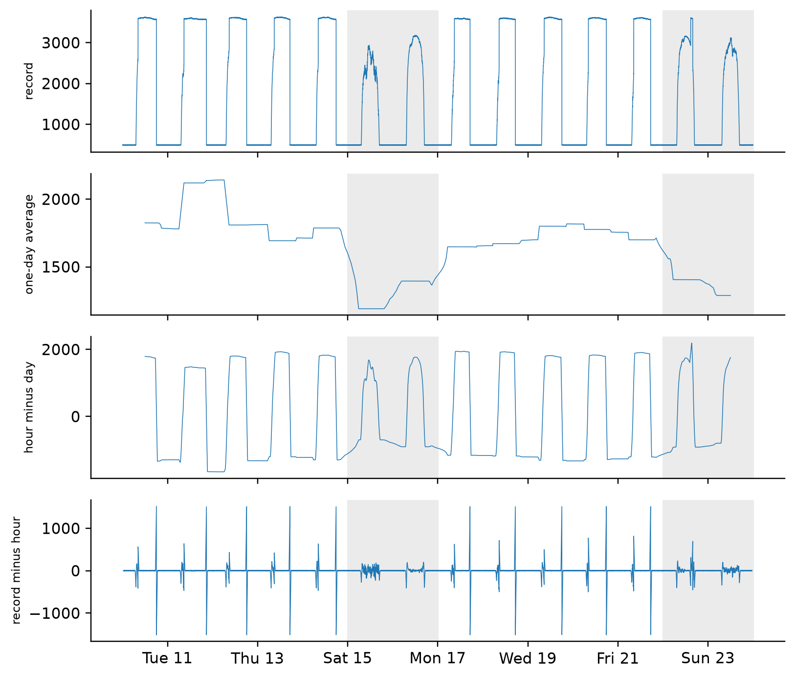
For the fourteen-day office record the natural windows are a day and an hour (Figure 9.4). The slow component, the one-day moving average, is the office’s level from day to day: it drops on both weekends, to about 1350 codes against 1680 to 1850 on weekdays, and it bulges on Tuesday 11 November, the evening the lights were left on in this fourteen-day record. The middle component is each day’s own cycle of darkness, daylight, and lamps. The fast component holds everything that happens within an hour. At night it is pure noise, with a standard deviation of 4.0 codes, the kit’s noise from Section 9.3.1 recovered by a different route; during the day it is dominated by the moments the lights switched, which are real events that happen to be fast. Fast does not mean noise; it means faster than the window.
Figure 9.4: The fourteen-day record split by centered moving averages over one day and one hour. From the top: the record; the one-day average (slow), which drops on the weekends (shaded) and bulges on the Tuesday evening the lights were left on; the one-hour average minus the one-day average (each day’s cycle); and the record minus the one-hour average (everything faster than an hour: noise at night, light switches by day). The three lower panels add up to the top one.
In pandas
import pandas as pdy = pd.read_csv("data/room_light_14d.csv", parse_dates=["timestamp_utc"], index_col="timestamp_utc")["adc_code"]day = y.rolling(1441, center=True).mean() # one-day average (slow)hour = y.rolling(61, center=True).mean() # one-hour averagemiddle, fast = hour - day, y - hour # y = day + middle + fast
Splitting by time scale keeps each day’s own cycle, which is right for finding what happened on a particular day and wrong for asking what a typical day looks like. Classical decomposition asks the second question: it replaces the within-day component with the one cycle that repeats, averaged over all the days, and leaves each day’s departure from it in the residual.
The additive decomposition writes each sample as \[
y_t = T_t + S_t + R_t,
\tag{9.19}\] a trend-cycle\(T_t\) that changes slowly, a seasonal component \(S_t\) that repeats with a known period of \(\tau\) samples, and a residual\(R_t\)(Hyndman and Athanasopoulos 2021, sec. 3.2). (This residual is not the one of Section 9.5.1, which subtracted only a rolling median.) The phase of a sample is its position within the cycle: for a daily cycle sampled once a minute, its minute of the day, from 0 to 1439. Classical decomposition estimates the three components in three steps (Hyndman and Athanasopoulos 2021, sec. 3.4):
The trend is a centered moving average one period wide, which averages exactly one sample at every phase of the cycle and so cancels the cycle. When \(\tau\) is even no window of \(\tau\) samples has a middle sample, and the standard fix is the \(2\times\tau\) moving average: \(\tau+1\) samples, the two end ones weighted \(1/(2\tau)\) and the rest \(1/\tau\), which is the average of the two \(\tau\)-sample windows either side of the center. Here \(\tau = 1440\) minutes.
The seasonal component at each phase is the average of the detrended values \(y_t - T_t\) at that phase, shifted so that the component sums to zero over one period.
The residual is whatever remains: \(R_t = y_t - T_t - S_t\).
The trend is the slow component of Section 9.7.1 computed with a window of exactly one period, and the seasonal and residual follow from it by subtraction and averaging.
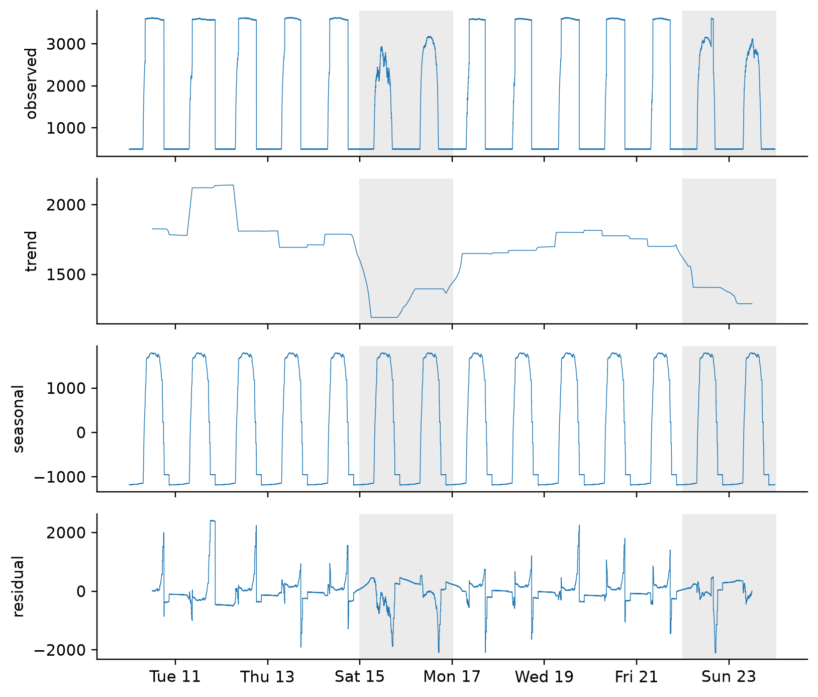
Figure 9.5: Classical additive decomposition of fourteen days of the office’s light record, with a daily period. The seasonal component is the average day. The weekly pattern, which a daily period cannot represent, lands in the trend, which dips on both weekends (shaded); the residual collects what no average day explains: the variable times the lights went on and off, and the Tuesday evening the lights were left on.
Three things are visible in Figure 9.5 that no single average would show. The seasonal component is the office’s average day: dark, a daylight hump, a lamp-lit plateau during working hours. The trend is not flat; it drops on both weekends, because a weekly pattern is invisible to a daily period and has to go somewhere. The residual is small most of the time and large at the edges of the working day, since the occupant does not arrive and leave at the same minute every day and the average day cannot follow, and it shows one long block on Tuesday evening, when the lights stayed on after everyone had left. That block is exactly the kind of anomaly the decomposition exists to expose, and in the raw record it is one bright evening among fourteen. Note also what the method cannot do: the trend is undefined for the first and last half day, because a one-day centered window does not fit there, and the seasonal shape is assumed to be the same every day, weekends included (Hyndman and Athanasopoulos 2021, sec. 3.4).
In pandas
import pandas as pdy = pd.read_csv("data/room_light_14d.csv", parse_dates=["timestamp_utc"], index_col="timestamp_utc")["adc_code"]y = y.tz_convert("America/New_York")trend = (y.rolling(1440).mean().rolling(2).mean() # the 2 x 1440 average, .shift(-720)) # centeredphase = y.index.hour *60+ y.index.minute # minute of the dayday_shape = (y - trend).groupby(phase).mean() # the average day...day_shape -= day_shape.mean() # ...summing to zeroseasonal = pd.Series(day_shape.reindex(phase).to_numpy(), index=y.index)residual = y - trend - seasonal
NoteOptional: STL and Multiplicative Decomposition
This material is optional: the classical decomposition above is what the course requires, but the decomposition routine you are most likely to find in a library is STL, and a sensor whose fluctuations grow with its level calls for the multiplicative form.
STL (Seasonal and Trend decomposition using Loess) replaces the moving averages with repeated locally weighted regressions (Hyndman and Athanasopoulos 2021, sec. 3.6). It lets the seasonal shape change slowly from one cycle to the next, can be made robust so that a few wild values do not distort the trend and seasonal estimates, and produces a trend at the ends of the record. Each of those answers a limitation visible in Figure 9.5. In Python it is statsmodels.tsa.seasonal.STL.
Multiplicative decomposition writes \(y_t = T_t \times S_t \times R_t\), which is the right model when the size of the seasonal swing scales with the level, as the daily swing of a building’s electricity demand grows with the building’s size (Hyndman and Athanasopoulos 2021, sec. 3.2). Taking logarithms turns it into the additive case, \(\log y_t = \log T_t + \log S_t + \log R_t\), so any additive method applies to the logged series. It needs strictly positive data, which light codes and power readings are and temperatures in degrees Celsius are not.
9.8 Virtual Sensors
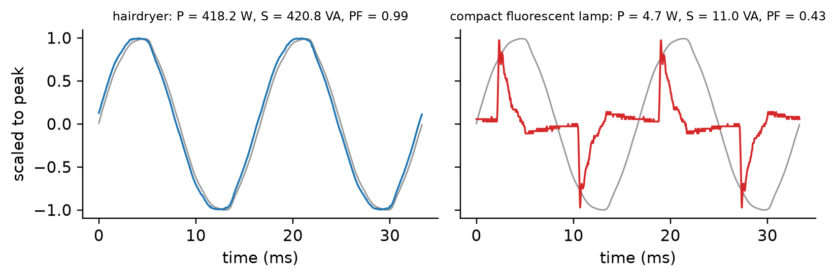
In many cases the quantity an engineer needs cannot be measured directly: the curvature of a beam, the rotation of a floor, the heat flux through a wall, the real power an appliance draws. A virtual sensor computes it from the sensors that can be installed, and it is a measurement like any other, with noise inherited from its inputs and, as this section shows on real voltage and current records, an accuracy that can be limited by its model rather than by its instruments.
A virtual sensor is defined by a function on the domain of the actual sensors: at each time \(i\), \[
z_i = f(x_i, y_i, \ldots),
\tag{9.20}\] where \(x_i, y_i, \ldots\) are the readings of the actual sensors at that time and \(z_i\) is the virtual reading. The function can be arithmetic: the average temperature of three rooms, \((T_1 + T_2 + T_3)/3\), or a building’s total electricity from its submeters, \(E_1 + E_2 + E_3\). It can be physics: the heat flux through a wall from its two surface temperatures and the wall’s thermal resistance per unit area \(R_{\text{w}}\), \(q = (T_{\text{in}} - T_{\text{out}})/R_{\text{w}}\). It can be a statistical model trained on data, which is where the MODELS third of this course is headed. In every case the output is used as if a sensor had measured it, which is exactly why it needs the same scrutiny.
A structural example makes the idea concrete. A beam bends, and what an engineer wants is its curvature\(\kappa\) (how sharply it bends) and its axial strain\(\varepsilon_A\) (how much it stretches as a whole). Neither can be measured directly, but strain can, with a gauge glued to the surface. Put one gauge on the top face and one on the bottom, a distance \(h\) apart and symmetric about the beam’s centroid, and use the fact that strain varies linearly through the depth of a beam in bending: with \(\eta\) measured upward from the centroid, \(\varepsilon(\eta) = \varepsilon_A - \kappa\,\eta\), taking tension as positive and a beam that sags as having positive curvature. The top gauge reads \(y_U = \varepsilon_A - \kappa h/2\) and the bottom one \(y_L = \varepsilon_A + \kappa h/2\), and solving for the two unknowns gives two virtual sensors: \[
z_C = \kappa = \frac{y_L - y_U}{h}, \qquad z_A = \varepsilon_A = \frac{y_U + y_L}{2}.
\tag{9.21}\] The same pattern runs through structural testing. When a concrete column is pushed back and forth by hydraulic actuators to study how it fails, the quantities in the plots that engineers read, the bending moment at the column’s base against its rotation, are both virtual: the moment computed from the measured actuator forces and their lever arms, the rotation from displacement transducers mounted across the base.
A virtual sensor. Its output inherits uncertainty from every measured input and every assumed constant, and its error from every way the model differs from the world.
Two requirements come with every virtual sensor. First, its inputs must describe the same moment: they usually come from different devices on different clocks, so a virtual sensor is only as good as the alignment of Section 9.6, and a heat flux computed from an indoor reading and an outdoor reading taken ten minutes apart is the flux of no moment in particular. Second, its inputs carry noise, and the noise passes through the function into the output, as the next subsection works out for the commonest case.
9.8.1 Linear Virtual Sensors and Their Noise
Most virtual sensors in structural and building monitoring are sums and differences of readings, and for those the noise of the output can be predicted exactly from the noise of the inputs. The prediction is the general averaging result of Section 9.3.3, and it says something that matters in practice: averaging sensors reduces noise, but differencing them adds it.
A linear virtual sensor weights \(m\) actual sensors: \[
z_i = \sum_{k=1}^{m} \alpha_k\, y_{k,i},
\tag{9.22}\] where \(y_{k,i}\) is the reading of sensor \(k\) at time \(i\) and the weight \(\alpha_k\) is the proportionality between the virtual sensor and actual sensor \(k\). The curvature of Equation 9.21 is one, with \(m = 2\) and weights \(\alpha_L = 1/h\), \(\alpha_U = -1/h\).
Now apply the white-noise model of Section 9.3.2 to every input: \(y_{k,i} = q_{k,i} + n_{k,i}\), where \(n_{k,i} \sim \mathcal{N}(0, \sigma_k^2)\), independent across sensors and across time. Because the function is linear, the virtual reading splits the same way, \(z_i = q_{z,i} + n_{z,i}\), into the virtual physical quantity \(q_{z,i} = \sum_k \alpha_k q_{k,i}\) and the virtual noise \(n_{z,i} = \sum_k \alpha_k n_{k,i}\). A sum of independent zero-mean normal variables is itself zero-mean and normal, so the virtual noise is white, \(n_{z,i} \sim \mathcal{N}(0, \sigma_z^2)\), with the variance of Equation 9.8: \[
\sigma_z^2 = \sum_{k=1}^{m} \alpha_k^2 \sigma_k^2 .
\tag{9.23}\] This is the noise level of the virtual sensor. For the average of \(m\) sensors of equal noise \(\sigma\), the weights are \(1/m\) and \(\sigma_z = \sigma/\sqrt{m}\), the averaging gain again. For the curvature, \(\sigma_z^2 = 2\sigma^2/h^2\): the difference of two readings is noisier than either reading, and when the two readings are nearly equal, as the strains on the two faces of a stiff beam under a small load can be, the difference is small and its noise is not, so the curvature can come out almost entirely noise. Equation 9.23 is the linear case of the propagation of uncertainty of Lecture 7 (Section 8.6), exact rather than approximate because nothing had to be linearized.
9.8.2 Worked Example: The Motion of a Two-Story Frame
A floor of a building moves in its own plane in three ways, two translations and a rotation, and no single accelerometer measures any of them, because each accelerometer measures one direction at one point and sees a mixture of all three. Four accelerometers per floor, placed with care, turn into virtual sensors that separate the mixture, with one sensor to spare as a check, and the frame of Lecture 6 is instrumented exactly this way.
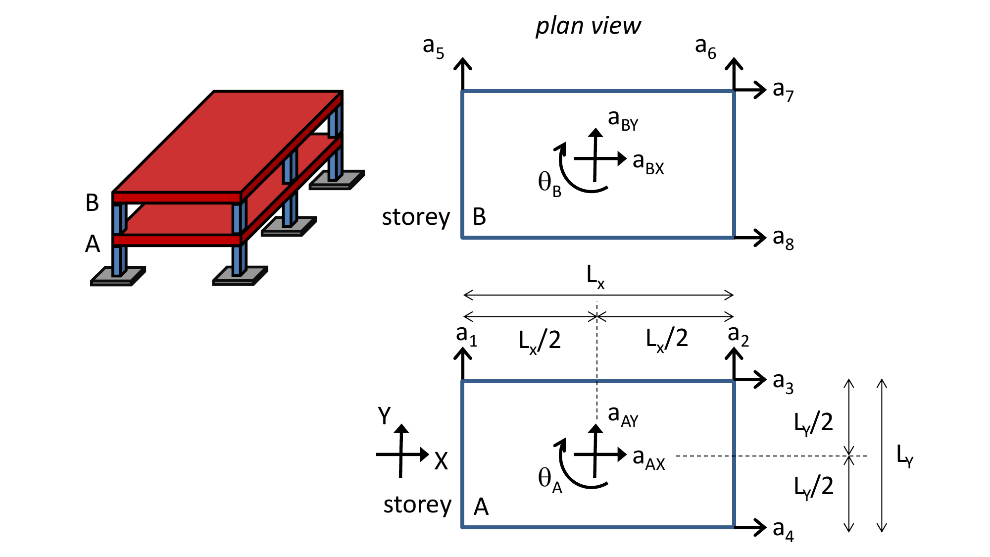
The record is the one analyzed in Lecture 6, collected by Matteo Pozzi and shared with permission: 25 s of the response of a two-story frame on a shaker table, sampled at 200 Hz on eight accelerometers, \(a_1\) through \(a_8\), and copied into this lecture’s data/ folder. On each story (Figure 9.6), two accelerometers measure \(Y\)-acceleration at the two ends of an edge of length \(L_X\), and two measure \(X\)-acceleration at the two ends of a perpendicular edge of length \(L_Y\).
Figure 9.6: The instrument layout of the two-story frame, in plan view: stories A (lower) and B (upper). On story B, \(a_5\) and \(a_6\) measure \(Y\)-acceleration at the two ends of an edge of length \(L_X\), and \(a_7\) and \(a_8\) measure \(X\)-acceleration at the two ends of a perpendicular edge of length \(L_Y\); story A repeats the pattern with \(a_1\) to \(a_4\). The virtual sensors are the accelerations \(a_X\) and \(a_Y\) of the center of each floor and its rotation \(\theta\), positive in the direction of the arrow. Layout courtesy of Matteo Pozzi.
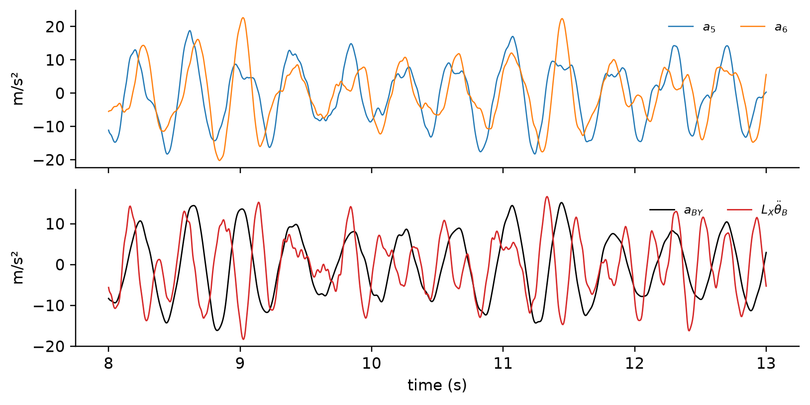
If a floor is rigid, the acceleration of any point on it follows from the acceleration of its center and its angular acceleration, and inverting that relation gives the virtual sensors. On story B, with rotation taken positive in the direction of the arrow in Figure 9.6, \[
a_{BY} = \frac{a_5 + a_6}{2}, \qquad
\ddot{\theta}_B = \frac{a_5 - a_6}{L_X}, \qquad
a_{BX} = a_7 - \ddot{\theta}_B\,\frac{L_Y}{2},
\tag{9.24}\] and on story A the same with \(a_1, a_2, a_3\) in place of \(a_5, a_6, a_7\). The average of the two \(Y\) sensors cancels the rotation, which moves the two ends of the edge by equal amounts in opposite directions, and leaves the translation of the center; their difference cancels the translation and leaves the rotation, here an angular acceleration because the inputs are accelerations; and the \(X\)-acceleration of the center is the reading of \(a_7\) corrected for the part of it caused by the floor’s rotation, since \(a_7\) sits a distance \(L_Y/2\) from the center line. All three are linear virtual sensors, and together they use three of the story’s four accelerometers.
Figure 9.7: Story B of the two-story frame, from 8 to 13 s. Top: the two \(Y\)-direction accelerometers, \(a_5\) and \(a_6\). Bottom: the virtual sensors built from them, the \(Y\)-acceleration of the floor’s center \(a_{BY} = (a_5 + a_6)/2\) and the rotational term \(L_X \ddot{\theta}_B = a_5 - a_6\), both in m/s². The two sensors disagree by nearly as much as they vary, so neither one alone measures the floor’s translation.
The record has no measurement noise in it, which makes it a clean test of Equation 9.23: add white noise of a known standard deviation, \(\sigma = 0.05\) m/s², independently to every channel, compute the virtual sensors from the noisy channels, and compare their noise with the prediction (Table 9.6).
Table 9.6: Noise of two virtual sensors of the frame, predicted by Equation 9.23 and measured on 5000 samples after adding white noise of \(\sigma = 0.05\) m/s² to every channel.
Virtual sensor
Weights \(\alpha_k\)
Predicted noise \(\sigma_z\) (m/s²)
Simulated noise (m/s²)
\(a_{BY} = (a_5 + a_6)/2\)
\(\tfrac12, \tfrac12\)
\(\sigma/\sqrt{2} = 0.0354\)
0.0351
\(L_X \ddot{\theta}_B = a_5 - a_6\)
\(1, -1\)
\(\sigma\sqrt{2} = 0.0707\)
0.0705
The average is quieter than either sensor and the difference is noisier, by factors of \(\sqrt{2}\) in each direction, as predicted. For \(a_{BX}\) as written in Equation 9.24, the weights are \(1\) on \(a_7\) and \(\mp L_Y/(2L_X)\) on \(a_5\) and \(a_6\), so \(\sigma_z^2 = \sigma^2\left[1 + L_Y^2/(2L_X^2)\right]\): the correction for rotation makes the translation of the center noisier than the raw reading it was computed from.
The fourth accelerometer changes that. \(a_8\) measures \(X\)-acceleration at the other end of the same edge as \(a_7\), a distance \(L_Y/2\) on the other side of the center line, so the same argument that gave \(a_{BY}\) gives a second way to compute the \(X\)-translation, and a second way to compute the rotation: \[
a_{BX} = \frac{a_7 + a_8}{2}, \qquad \ddot{\theta}_B = \frac{a_7 - a_8}{L_Y}.
\tag{9.25}\] The first has noise \(\sigma/\sqrt{2}\), quieter than \(a_7\) alone rather than noisier, which is the reason to install the fourth sensor. The second is redundant: the floor has three ways to move and four sensors to observe it, so one combination is a check rather than a measurement. If the floor really is rigid, the two rotation estimates must agree, so \(a_7 - a_8\) must be proportional to \(a_5 - a_6\) at every instant, with constant ratio \(L_Y/L_X\). In this record they are, on both stories, with a correlation of 1.000; a floor that flexed, or a sensor that slipped, would show up as a disagreement between them. A spare sensor turns an assumption of the model into something the data can test.
In pandas
import pandas as pda = pd.read_csv("data/SeismicResponse_noNoise.txt", sep="\t", header=None, names=[f"a{k}"for k inrange(1, 9)])a_BY = (a["a5"] + a["a6"]) /2# translation of story B's centerLx_theta_B = a["a5"] - a["a6"] # L_X times its angular accelerationa_BX = (a["a7"] + a["a8"]) /2# X-translation, from a7 and a8Ly_theta_B = a["a7"] - a["a8"] # rotation again: a rigid-floor checkLx_theta_B.corr(Ly_theta_B) # 1.000 if the floor is rigid
9.8.3 Real Power from Voltage and Current
The power an appliance draws looks easy to compute: multiply its voltage by its current. Do it with the usual one-number summaries of the two waveforms, and for the compact fluorescent lamp in this section’s data the answer is about two and a half times too high, while for the hairdryer beside it the same recipe is within one percent. The right answer averages the product of voltage and current sample by sample, and computing both answers on real appliance records turns the gap between them, the power factor, into something observed rather than asserted.
The records come from PLAID, a public dataset of appliance voltage and current waveforms collected in Pittsburgh homes (Gao et al. 2014). The ten used here, in data/plaid/, were recorded in one house in July 2013: five of a compact fluorescent lamp and five of a hairdryer, each two seconds long at 30 kHz, each starting with the appliance off and switching it on. The dataset’s own notes warn that some instances are not well calibrated, and one sign of that is visible in these files: the rms voltage over each whole record is exactly 120.000 V, in every one of them, which a real supply does not do, so the voltage has been scaled to its nominal value and its magnitude here is an assumption; its shape and timing are measurements.
Three quantities describe the power an AC load draws, and all of them use the rms (root-mean-square) value of a waveform, \(V_{\text{rms}} = \sqrt{\frac{1}{N}\sum_k v[k]^2}\) for \(N\) voltage samples \(v[k]\) (and likewise \(I_{\text{rms}}\) from the current samples \(i[k]\); in this subsection \(i\) is the current, as is standard in electrical work, and \(k\) counts samples), the steady value that would deliver the same power to a resistor. The real power\(P = \frac{1}{N}\sum_k v[k]\, i[k]\) is the average of the instantaneous power, voltage times current at each sample; it is what turns into heat and light, and what the utility bills as energy. The apparent power\(S = V_{\text{rms}} I_{\text{rms}}\), in volt-amperes, is what the wiring has to carry. Their ratio is the power factor, \[
\text{PF} = \frac{P}{S} = \frac{\frac{1}{N}\sum_k v[k]\, i[k]}{\sqrt{\frac{1}{N}\sum_k v[k]^2}\,\sqrt{\frac{1}{N}\sum_k i[k]^2}},
\tag{9.26}\] which is 1 for a purely resistive load, whose current is a scaled copy of the voltage, and less than 1 whenever the current is shifted in time or distorted in shape. Every average is taken over a whole number of mains cycles, for the reason Lecture 6 gave: a partial cycle leaves a piece of the oscillation in the mean. Here the averages use the last 60 complete cycles of each record, one second of steady operation well after the switch-on.
Table 9.7: Real power, apparent power, and power factor over one second of steady operation, ranges over the five records of each appliance from PLAID.
Appliance
Real power \(P\) (W)
Apparent power \(S\) (VA)
Power factor
Peak current (A)
Hairdryer
417.2 to 418.2
419.7 to 420.8
0.994 to 0.994
4.9 to 4.9
Compact fluorescent lamp
4.0 to 4.7
10.5 to 11.0
0.385 to 0.428
0.4 to 0.4
Figure 9.8: Two mains cycles of voltage (gray) and current (colored) for a hairdryer and a compact fluorescent lamp from PLAID, each scaled to its own peak. The hairdryer’s current follows the voltage, and its power factor is close to 1. The lamp draws its current in a sharp pulse early in each half-cycle, while the voltage is still rising, followed by a decaying tail; most of its rms current does no useful work, and its power factor is about 0.4.
Table 9.7 holds the whole argument. For the hairdryer, \(V_{\text{rms}} I_{\text{rms}}\) is within 0.6% of the real power; for the lamp it is 2.3 to 2.6 times too high. The instruments are equally good in both cases, since they are the same instruments in the same house. What differs is whether the model \(P = V_{\text{rms}} I_{\text{rms}}\) describes the load, and for a lamp that draws its current in short pulses (Figure 9.8) it does not.
9.8.4 When the Model Is the Weak Link
A current transformer such as the CR3110-3000, whose datasheet this course has used as a running example, measures current alone, so a virtual power sensor built on one has to assume the voltage, and the machinery of Lecture 7 will cheerfully return an uncertainty for an answer that is wrong for an entirely different reason. This section separates uncertainty that propagates from the inputs from error introduced by a model being wrong, and shows the same failure in a virtual sensor where the arithmetic is trivial and the model is indefensible.
With a current transformer and nothing else, the natural estimate is \(\hat{P} = V_{\text{nom}} I_{\text{rms}}\): the nominal 120 V times the measured current. Its uncertainty budget, built as in Lecture 7, has two inputs. The current carries the transformer’s and the converter’s uncertainty. The voltage is not measured, so it enters as a Type B term, a statement about how far the supply might be from nominal; if it could be anywhere within \(\pm 5\%\), a uniform distribution gives a standard uncertainty of \(5\%/\sqrt{3} = 2.9\%\). Propagate both and the budget reports a few percent, honestly. For the hairdryer that is also the error. For the lamp the error is between 134% and 160%, and nothing in the budget hints at it, because the budget propagates the uncertainty of every input that was listed, and the model silently fixed one more at a value nobody checked: the power factor, at 1. An input assumed away contributes nothing to the uncertainty and everything to the error.
The two-day office record has a virtual sensor of the same kind hiding in it. “The room is occupied when the PIR sensor reads 1” is a model, and a tempting one, since the arithmetic is trivial. It is also wrong in both directions: the PIR read 0 on 47% of the minutes when somebody was in the room, because people sit still, and on Monday evening of the two-day record the room was bright for 280 minutes after its occupant had gone home. Neither failure is a measurement error; both sensors did exactly what they are specified to do. The model is the weak link, and the only defense is to test it against something independent, which for occupancy usually means a person counting.
9.9 Storing Time Series
A hundred kits sampling once a minute for a year is a number worth computing before choosing a file format, because the obvious choice costs several times more than it has to. Row-oriented text, column-oriented binary, and purpose-built time-series databases trade size against read speed and interoperability in different directions, and this section measures the first two on the fourteen-day record.
CSV is text, one row per line, each value written out as characters. Anything can read it, a person included, and that is its whole case. It is also large, because a four-digit code costs four bytes plus a comma, and a timestamp costs twenty; and it is slow to read, because every value has to be parsed back from characters, and nothing in the file says what type a column is. Compressing the file with a general-purpose compressor such as gzip shrinks it a great deal, since sensor records repeat themselves, but keeps it just as slow to read.
Parquet is a binary, column-oriented format: the file stores all of one column together, then the next, each with its type recorded and each compressed on its own (The Apache Software Foundation, n.d.). A column of timestamps one minute apart, or of ADC codes that change by a few counts, compresses far better on its own than interleaved with other columns, and a program that needs one column reads only that column. The cost is interoperability: a person cannot read a Parquet file, and a program needs a library to, though every major data tool now has one.
Table 9.8: The fourteen-day record (20,160 rows) in four formats, all lossless. Sizes and read times are relative to plain CSV; read times include parsing the timestamps.
Format
Size (kB)
Relative size
Relative read time
Readable by
CSV
553
1.000
1.00
anything, even a person
CSV, gzip-compressed
76
0.137
0.98
anything, once unzipped
Parquet, default settings
197
0.356
0.02
Parquet-aware programs
Parquet, delta-encoded columns
19
0.035
0.02
Parquet-aware programs
Table 9.8 has a surprise in it. Compression shrinks the CSV about sevenfold, and it reads no faster, since the file must be decompressed and then parsed exactly as before. Parquet with its default settings reads more than ten times faster, because there is nothing to parse, but it is larger than the compressed CSV: by default it stores each timestamp as a full eight-byte integer, and twenty thousand of them are most of the file. Tell it that the timestamps and codes change by small steps from one row to the next, so that it stores those steps instead of the values (delta encoding), and the same data takes a quarter of the space of the compressed CSV while still reading as fast. Why storing differences saves so much is the subject of Lecture 12; the lesson here is that the format is a choice with several dimensions, and its defaults are not the answer. Scaled up, the choice stops being a detail: at 27.4 bytes a row, a hundred kits writing one row a minute for a year produce about 1.4 GB of CSV, and the delta-encoded Parquet version of the same data about 0.05 GB.
The fourteen-day file is in the synchronous form of Section 9.2.1, one row per scan; the single-table form of the same data would repeat each timestamp once per sensor and carry the metadata on every row, about three and a half times the size before any compression. A time-series database goes one step further. It is built around the shape every record in this lecture has, a series identifier, a timestamp, and a few values, and it stores points sorted by time, compresses them with methods designed for slowly changing, regularly spaced values, and usually offers downsampling and retention rules as built-in operations: keep the one-minute data for a month and the hourly means forever. InfluxDB and TimescaleDB, an extension to the PostgreSQL database, are two widely used examples. What such a system adds over a file is the ability to ask questions of the data efficiently, which is where the next lectures go: Lectures 9 through 11 are about databases and the language for querying them, and Lecture 12 explains why the encodings that make Parquet small work at all.
In pandas
import pandas as pdd = pd.read_csv("data/room_light_14d.csv")df = pd.DataFrame({"timestamp_utc": pd.to_datetime(d["timestamp_utc"]),"adc_code": d["adc_code"].astype("int16"),"pir_state": d["pir_state"].astype(bool)})df.to_csv("room.csv", index=False)df.to_csv("room.csv.gz", index=False) # gzip, from the file namedf.to_parquet("room.parquet", index=False) # needs pyarrowdelta = {"timestamp_utc": "DELTA_BINARY_PACKED","adc_code": "DELTA_BINARY_PACKED"} # store the stepsdf.to_parquet("room.parquet", index=False, use_dictionary=False, column_encoding=delta)pd.read_parquet("room.parquet", columns=["adc_code"]) # one column only
9.10 Putting It All Together
A sensor record is data only when it says what was measured, by which sensor, and when, and the first job with any record is to read its layout and its clocks. Every later step then rests on a model of noise: averaging and smoothing shrink it by the square root of what they average, at the price of blurring what changes; cleaning is a series of claims about what happened while nobody was looking, each worth stating, and outlier rules flag what is surprising rather than what is wrong; decomposition splits a record by time scale; and virtual sensors combine many sensors into quantities none of them measures, inheriting their noise by a rule simple enough to compute and a model that can fail where no instrument does. Storing the result is a trade between the person who might read it and the program that will. This lecture moved the course from signals to data, and the next four put that data where it can be queried.
9.11 Exercises
A naive local log from a Pittsburgh building contains the line 2025-11-02 01:30:00, 812. Give both instants in UTC it could refer to, and name two pieces of information that, if the record had them, would decide between the two.
TipSolution
Before the clocks went back, 01:30 EDT is 05:30 UTC; after, 01:30 EST is 06:30 UTC. A monotonic device clock such as time_ms would decide it, since the second 01:30 comes an hour of device time after the first; so would an explicit offset on the stamp (-04:00 or -05:00), and so would the position of the line among neighbours known to be in order. The lasting fix is to write UTC with an offset in the first place.
The kit’s night-time noise is \(\sigma = 3.9\) codes.
How many readings of the dark room must be averaged for the standard deviation of the average to be 0.5 codes?
At 07:00 on Monday the light is rising. Why would averaging the same number of consecutive readings then not give an estimate that good?
TipSolution
From Equation 9.7, \(\sigma/\sqrt{N} \le 0.5\) requires \(N \ge (3.9/0.5)^2 = 60.8\), so 61 readings, an hour of data.
The derivation assumed a constant quantity, \(y_i = L + n_i\). At dawn the light rises during the hour, so the average blends different light levels. Its noise is still about 0.5 codes, but it estimates the light averaged over the hour, not the light at any moment, and a reading at the end of that hour can differ from it by hundreds of codes.
A careful student records the same steady voltage \(N = 500\) times.
Find the critical distance \(z_c\) of Chauvenet’s criterion for this \(N\).
The student then applies the criterion to a week of outdoor air temperature logged every twenty minutes, also \(N = 504\). Which of the criterion’s assumptions fail, and what would you expect it to reject?
The readings are neither identically distributed nor scattered about a constant mean: they follow a daily cycle and whatever weather came through, and successive readings are strongly correlated, not independent. The standard deviation is dominated by that structure, so, as with the light record, the criterion will likely reject nothing, including real sensor faults; remove the daily cycle first (a rolling median, or the seasonal component of a decomposition) and test the residual.
A facilities manager asks, for each day, how many hours the office’s lights were on and how many hours the room was occupied, from the two-day record. Propose a resampling rule for each question and state what your rule assumes about the gaps.
TipSolution
For lights, classify each sample as lit or unlit by a threshold between the night level and the lamp level (a code around 3400 separates them in this record: daylight alone never lifts the reading above about 3200, and the lamps never let it fall below about 3550), then count lit minutes per day and report the count of recorded minutes alongside it; the Monday outage is reported as unknown, not as dark. For occupancy, the PIR channel cannot answer the question directly, because it reads 0 on many occupied minutes; the defensible summary is “minutes with any motion within the last \(k\) minutes,” with \(k\) stated, and the answer should be labeled as motion, not occupancy. Neither rule fills the gaps, and both carry the coverage with the answer.
On story A of the two-story frame, \(L_X = 2 L_Y\), and each accelerometer has white noise of standard deviation \(\sigma\), independent of the others.
Find the noise standard deviation of \(a_{AY}\) and of \(\ddot{\theta}_A\) from Equation 9.24.
Compare the noise of the two ways of computing \(a_{AX}\): from \(a_3\) corrected for rotation (Equation 9.24), and as \((a_3 + a_4)/2\) (Equation 9.25).
TipSolution
By Equation 9.23: \(a_{AY} = (a_1 + a_2)/2\) has weights \(\tfrac12, \tfrac12\) and noise \(\sigma/\sqrt{2} \approx 0.71\,\sigma\). \(\ddot{\theta}_A = (a_1 - a_2)/L_X\) has weights \(\pm 1/L_X\) and noise \(\sqrt{2}\,\sigma/L_X\), in rad/s² (its units differ from the sensors’).
\(a_{AX} = a_3 - \ddot{\theta}_A L_Y/2\) has weights \(1\) on \(a_3\) and \(\mp L_Y/(2L_X) = \mp\tfrac14\) on \(a_1\) and \(a_2\), so its noise is \(\sigma\sqrt{1 + 2/16} = \sqrt{9/8}\,\sigma \approx 1.06\,\sigma\), noisier than \(a_3\) alone. \((a_3 + a_4)/2\) has noise \(\sigma/\sqrt{2} \approx 0.71\,\sigma\), so the rotation-corrected estimate is exactly 1.5 times as noisy, and the average needs no knowledge of \(L_X\) or \(L_Y\). The fourth sensor buys both a quieter translation and a check on the rotation.
Using Table 9.7, a household runs the compact fluorescent lamp four hours a day for a year.
Estimate the energy it uses, in kWh.
An energy auditor with only a clamp-on current meter estimates the lamp’s power as \(120\ \text{V} \times I_{\text{rms}}\). What would the auditor report, and which of the two numbers does the utility bill?
TipSolution
With \(P \approx 4.4\) W, energy is \(4.4\ \text{W} \times 4\ \text{h} \times 365 \approx 6.4\) kWh a year.
The auditor measures apparent power, about \(11\) VA for this lamp, and would report about \(16\) kWh, about two and a half times the real figure. The utility bills real energy, the integral of \(P\). The apparent power is not meaningless, though: it is what the wiring carries, and a building full of such lamps loads its transformers more than its energy bill suggests.
A campus deploys 300 kits, each writing one row a minute in the format of the fourteen-day record, for a year. Using Table 9.8, estimate the storage required as CSV and as Parquet, and say what besides size you would weigh before choosing.
TipSolution
One kit-year is \(525{,}600\) rows. At the fourteen-day file’s 27.4 bytes a row, 300 kit-years of CSV is about 4.3 GB, and at the delta-encoded Parquet file’s 0.035 of the CSV size it is about 0.15 GB. Size is not the deciding factor at this scale, since either fits on a laptop; what matters is who reads the data (people and spreadsheets favor CSV; analysis programs favor Parquet), how it will be queried (by time range and by kit, which favors a sorted, columnar layout or a time-series database), and how the data’s provenance and quality flags travel with it.
(Optional, depends on the optional section.) Hourly electricity demand of a campus building has a daily swing of about 20% of its level, and its level rises by half over the summer. Explain why an additive decomposition would misplace part of the daily pattern, and how you would decompose it instead.
TipSolution
An additive model assumes the daily swing has the same size in watts all year, so when the level rises in summer, the larger summer swing does not fit the average seasonal component and its excess appears in the residual as a spurious daily pattern. A multiplicative model, \(y_t = T_t \times S_t \times R_t\), assumes a swing of constant proportion, which matches a 20% swing; decompose \(\log y_t\) additively, or use a method such as STL on the logged series.
The PLAID dataset, with more than a thousand appliance records, for anyone who wants to build a better virtual sensor than \(V_{\text{rms}} I_{\text{rms}}\).
Wikipedia’s articles on the Gaussian process and the Kalman filter, the principled ways to estimate values that were not observed, with an uncertainty attached to each.
The IANA time zone database, the source every operating system and pandas consult for rules such as the one that made Sunday 2 November 2025 twenty-five hours long in Pittsburgh.
9.13 References
McKinney (2022) (Ch. 11, especially §11.4 Time Zone Handling, §11.6 Resampling and Frequency Conversion, §11.7 Moving Window Functions)
Hyndman and Athanasopoulos (2021) (Ch. 3, especially §3.3 Moving averages, §3.4 Classical decomposition, §3.6 STL decomposition)
Gao, Jingkun, Suman Giri, Emre Can Kara, and Mario Bergés. 2014. “PLAID: A Public Dataset of High-Resolution Electrical Appliance Measurements for Load Identification Research: Demo Abstract.”Proceedings of the 1st ACM Conference on Embedded Systems for Energy-Efficient Buildings (BuildSys ’14) (New York, NY, USA), 198–99. https://doi.org/10.1145/2674061.2675032.
Hyndman, Rob J., and George Athanasopoulos. 2021. Forecasting: Principles and Practice. 3rd ed. OTexts. https://otexts.com/fpp3/.
McKinney, Wes. 2022. Python for Data Analysis: Data Wrangling with Pandas, NumPy, and Jupyter. 3rd ed. O’Reilly Media. https://wesmckinney.com/book/.
They are rows 281, 822, 1301, 1769, and 2448: 03:41, 13:27, and 21:14 on Sunday and 05:02 and 19:48 on Monday, by the laptop’s clock. Each is one reading far from its neighbours; the last one reads 4095, the converter’s largest code.↩︎