3  Lecture 02: Physical Principles of Sensing

3.1 Lecture Overview

NoteLearning Objectives

By the end of this lecture, students should be able to:

• Describe the measurement chain that links a physical quantity of interest (the measurand) to a recorded value: transduction, conditioning, digitization, and storage
• Classify common transduction principles (resistive, capacitive, inductive, piezoelectric, thermoelectric, optical) and give an example sensor for each
• Interpret the static characteristics reported in a sensor datasheet: sensitivity, range, resolution, linearity, hysteresis, and drift
• Select an appropriate sensing modality for common measurands in civil and environmental engineering (strain, displacement, acceleration, temperature, humidity, flow, water quality)
• Explain how the physics of a transducer constrains the quality and interpretation of the data it produces

NoteTopics Covered

• Measurements and instruments: from rulers and scales to digital instruments
• The measurement chain and the anatomy of a sensor
• Transduction principles and the physics inside common sensors
• Static characteristics on a datasheet
• Matching sensors to CEE measurands
• How transducer physics shapes the data downstream

3.2 Measurements and Instruments

Every claim in engineering rests on a measurement: a number, attached to a physical quantity, by some procedure. The deflection limit you checked in a design code, the concrete strength you accepted from the lab, the “the building used 12% less energy” line in a report — each is only as trustworthy as the procedure that produced the number. And yet, when data arrive in a spreadsheet, we tend to treat them as facts rather than as the output of a device somebody designed. This course is about closing that gap, and this first lecture starts with the most basic question: what is a measurement, and what is the thing that makes one?

A measurement is the assignment of a value to a quantity by comparing it against a reference. When you say a beam is 3.2 m long, you are saying it matches 3.2 copies of a reference length. Nothing in that statement is automatic: someone had to decide what the reference is, build an object that embodies it, and define a comparison procedure whose result you can trust. The device that carries out that comparison is an instrument.

3.2.1 Everyday Instruments

The instruments you already own show the whole story. A ruler looks like a stick with marks on it, but consider the decisions behind it: a range (30 cm, because that fits a desk), a resolution (millimeter marks, because your eye cannot reliably split them), a material chosen so that the marks do not move (steel or a stable plastic, not rubber), and a manufacturing step in which the marks were printed against a more accurate reference, that is, a calibration. Consider also how it can be wrong: the marks were printed with some tolerance, the plastic expands on a hot day, the end wears down after years of use so the zero is no longer at zero. Every one of those failure modes has a name on a datasheet — accuracy, drift, offset — and we will meet them formally in Section 3.5. The ruler has them too; it simply does not come with a datasheet.

A bathroom scale is a richer example because you cannot see the reference. Inside is a spring (in old ones) or a strain-sensing element (in new ones) whose deformation under your weight is compared, through a mechanism or a circuit, against the behavior the designer measured in the factory with known masses. That comparison is stored in the scale — as the shape of a dial, or as a few numbers in a chip — and it is only valid as long as the spring behaves as it did in the factory. Leave the scale in a damp bathroom for a decade and the stored comparison quietly stops being true. This is why serious instruments get re-calibrated on a schedule, and why “the sensor said so” is never the end of an argument.

TipActive Learning: An Instrument You Own

Pick either a ruler or a bathroom scale and write down, in a few lines each: what it was designed to measure and over what range; what its resolution is and what limits it; how it was calibrated (what was the reference?); and at least three distinct ways it could give you a wrong number. Keep your list — by the end of Section 3.5 you should be able to name every item on it with a datasheet term.

3.2.2 Modern Instruments

A digital thermometer does the same job as a mercury one, but open it up and you find a very different object: a tiny element whose electrical resistance depends on temperature, a circuit that turns that resistance into a voltage, a chip that turns the voltage into a number, a display, a battery, and maybe a radio. Only one of those parts actually responds to temperature. The rest exist to make the response usable — to amplify it, to digitize it, to show it, to send it — and every one of them can add error of its own.

That is the picture of a modern instrument worth keeping in mind for the entire course: a transducer surrounded by supporting components. The transducer is where physics happens; the supporting components are where engineering happens; the data you eventually analyze are the product of both. When the course description says a model’s performance “depends on how data are measured,” this is what it means concretely. If you want to trust a model built on sensor data, you have to understand what the transducer could and could not see, and what the chain around it did to the signal on the way to storage. The next section names the links of that chain; the rest of the lecture is about the transducer at its head.

3.3 The Measurement Chain

Suppose a temperature reading in your building database is wrong. Where is the fault? It could be in the probe itself, in the wiring that connects it, in the amplifier, in the analog-to-digital converter, in the logger that timestamps it, or in the database that stores it. Unless you can name those stages, you cannot even begin to debug, and you certainly cannot say which errors a downstream model should worry about. The measurement chain is that list of stages (Figure 3.1), and it doubles as the map of the SENSORS third of this course: this lecture covers the first block, Lectures 3–5 cover the middle, and the DATA third picks up where the chain ends.

Figure 3.1: The measurement chain of a typical instrument. The double arrow between sensor and signal conditioner reflects that many sensors need an excitation signal supplied to them.

3.3.1 What Is a Sensor?

A thermistor does not output “temperature.” It outputs a resistance, which something else must read. That small observation forces us to be precise about words. Following Fraden (2016), we will say:

A sensor is a device that receives a stimulus and responds with an electrical signal.

The stimulus (or measurand, when we want to stress that we intend to quantify it) is the physical quantity being sensed: temperature, strain, light, current. The response is electrical — a voltage, a current, a charge, a resistance — because electrical signals are what circuits, converters, and computers can handle. A sensor is therefore a translator from the physical world into the electrical one.

A transducer is the more general device: it converts energy from one form into another, in any direction. A loudspeaker is a transducer (electrical → acoustic); so is an electric motor (electrical → mechanical); neither is a sensor. Transducers that go the other way, into electrical energy, are sensors. So every sensor is a transducer, but not every transducer is a sensor — and in engineering practice you will hear the two used interchangeably, which is fine as long as you know what the speaker means. Transducers that go from electrical to physical are usually called actuators, and you will meet plenty of them in control systems.

One more subtlety matters for us. Many sensors are really a chain of transducers ending in one that produces electricity. A fiber-optic pressure sensor turns pressure into strain in a fiber, strain into a change of refractive index, refractive index into a change in light intensity, and only then light into current at a photodiode. Fraden calls the last stage a direct sensor and the whole assembly a complex sensor. We will meet the most important example of this pattern, the accelerometer, at the end of Section 3.4.

3.3.2 Classifying Sensors

A catalog contains thousands of sensors. Without a few organizing axes there is no way to reason about which family suits a job, so here are the three that Fraden proposes and that we will use throughout (Fraden 2016, Ch. 1):

1. By energy source: passive or active. A passive sensor generates its electrical signal directly from the stimulus, with no external power: a thermocouple, a photodiode, a piezoelectric crystal. An active sensor needs an excitation signal, which the stimulus then modulates: a thermistor is just a resistor until you pass a current through it, and a strain gauge likewise. Active sensors are sometimes called parametric because a parameter of theirs (resistance, capacitance) is what changes. This axis matters practically: passive sensors can run without a supply, active ones need a circuit that provides one, and (as we will see in Section 3.7) that excitation can itself disturb the measurement. The double arrow in Figure 3.1 is that excitation.

2. By reference: absolute or relative. An absolute sensor responds relative to a fixed physical scale independent of conditions — a thermistor’s resistance is a function of absolute temperature. A relative sensor responds to the difference from some baseline: a thermocouple produces a voltage that depends on the temperature difference between its two junctions, so it cannot tell you a temperature without a known reference. Gauge versus absolute pressure sensors are the other classic pair.

3. By characteristics. Fraden’s remaining tables list the ways a sensor can be described: by its specifications (the datasheet numbers of Section 3.5), by material, by detection means (electric, magnetic, thermal, mechanical, radiation, …), by conversion phenomenon (thermoelectric, photoelectric, electromagnetic, …), by field of application, and by stimulus. The conversion phenomenon is what we will call the transduction principle in Section 3.4 — arguably the single most informative label a sensor can carry.

3.3.3 Three Sensors Up Close

Definitions stick only once you have applied them to devices you could actually buy, so here are the three we will keep returning to. Each is cheap, common in student projects, and comes with a real datasheet you should open now (links in Table 3.1).

Accelerometer: Analog Devices ADXL335. A three-axis accelerometer on a 4 mm × 4 mm chip. Inside is a polysilicon proof mass suspended on springs above a silicon wafer; its motion unbalances a differential capacitor formed between plates on the mass and fixed plates around it, and on-chip electronics turn that imbalance into three voltages, one per axis. It needs a supply (1.8–3.6 V) — an active sensor — and it responds to acceleration relative to free fall, so it reads 1 g sitting on the table: an absolute sensor. Its conversion phenomenon is capacitive, its stimulus mechanical. At 3 V it produces about 300 mV per g over a ±3 g range.

Photoresistor: GL5528 CdS cell. A disc of cadmium sulfide whose resistance falls as light falls on it: from more than 1 MΩ in darkness to roughly 8–20 kΩ at 10 lux. It generates nothing by itself — you must pass a current through it — so it is active; it responds to light level referenced to darkness, so absolute. Its detection means is optical, but its conversion phenomenon is photoconductive: the output is a resistance, which is why we will file it under resistive in Section 3.4. It is slow (rise and fall times of tens of milliseconds) and its resistance also depends on temperature, two facts that will matter later.

Split-core current transformer: CR Magnetics CR3110-3000. A hinged iron ring that clamps around a live conductor without cutting it. The alternating current in the conductor creates an alternating magnetic field in the ring, which induces a current in a coil of about 3000 turns wound on it; the induced current is the primary current divided by the turns ratio. The energy comes from the conductor being measured, so the CT is passive; it reports current referenced to zero, so absolute. Its conversion phenomenon is electromagnetic induction — inductive in our scheme — and it only works for AC (20 Hz to 1 kHz on this part), which is the kind of limitation the physics imposes and a datasheet quietly records.

Table 3.1: The three sensors used as running examples, classified along the axes of Section 3.3.2.

Sensor	Part	Stimulus → output	Energy	Reference	Principle	Datasheet
Accelerometer	ADXL335	acceleration → voltage	active	absolute	capacitive	Analog Devices
Photoresistor	GL5528	illuminance → resistance	active	absolute	resistive (photoconductive)	GL55 series sheet
Current transformer	CR3110-3000	AC current → current	passive	absolute	inductive	CR Magnetics CR3100 series

3.3.4 The Rest of the Chain

A raw sensor signal is usually the wrong size and the wrong shape: millivolts when the converter wants volts, a resistance when the converter wants a voltage, a clean signal riding on noise picked up by a meter of cable. None of it can go straight into a display or a database. The rest of the chain exists to fix that, and each link gets a lecture of its own; here we only fix what each is responsible for.

The signal conditioner turns the sensor’s output into a clean voltage of convenient size: it supplies excitation to active sensors, converts resistance or current to voltage, amplifies, filters, and isolates (Lectures 3 and 5). Signal processing is everything done to that voltage before it becomes information: in a digital instrument, that means sampling and analog-to-digital conversion (Lecture 4), followed by whatever arithmetic runs on the resulting numbers — from a moving average to a full frequency analysis (Lecture 6). Finally, the result is displayed, transmitted, or stored, and the moment it is stored it becomes data — the subject of the second third of the course.

Figure 3.2 and Figure 3.3 show the two classic ways the chain is realized. In an analog instrument everything stays a continuous voltage until a needle or a chart recorder shows it; in a digital one an analog-to-digital converter sits in the middle and a computer does the rest. Nearly everything you will build is the second kind, but the first is worth knowing because the analog front end — input circuit, preamplifier, filters — is still there in front of every converter.

Figure 3.2: A typical analog instrument.

Figure 3.3: A typical digital instrument.

3.4 Transduction Principles: The Physics Inside

The three sensors we just met look nothing alike: a silicon chip, a blob of cadmium sulfide, a hinged iron ring. Yet each is a single physical effect that turns its stimulus into an electrical quantity, and knowing which effect predicts a great deal — how fast the sensor is, whether it needs power, how it will react to temperature, what circuit it needs — before you read a single line of its datasheet. Six effects cover most of what a civil or environmental engineer will ever deploy. For each we ask the same four things: what problem it solves best, what relation governs it, which electrical quantity changes, and where it shows up in our field.

3.4.1 Resistive

The cheapest way to sense strain or temperature is to let the stimulus change a resistance, because a resistance is the easiest electrical quantity to read with a simple circuit (Lecture 3 will show you exactly how). The resistance of a conductor of resistivity \(\rho\), length \(l\), and cross-sectional area \(a\) is

\[ R = \rho\,\frac{l}{a}. \tag{3.1}\]

Anything that changes \(l\), \(a\), or \(\rho\) changes \(R\). Stretch the conductor and \(l\) grows while \(a\) shrinks: that is the strain gauge, the workhorse of structural monitoring. How much \(R\) changes per unit strain is the gauge factor \(\text{GF} = (\Delta R/R)/\varepsilon\). A quick way to estimate it is to assume the conductor keeps its volume \(v = l\,a\) as it stretches, so \(R = \rho\,l^2/v\) and \(\mathrm{d}R/\mathrm{d}l = 2\rho\,l/v\), which gives \(\text{GF} = 2\) exactly. The honest version is \(\text{GF} = 1 + 2\nu + (\Delta\rho/\rho)/\varepsilon\), where \(\nu\) is Poisson’s ratio: the geometric part alone is \(1.6\) for \(\nu = 0.3\), the constant-volume shortcut corresponds to \(\nu = 0.5\), and the last term — the piezoresistive effect, the change of resistivity itself with strain — supplies the rest. Metal foil gauges land near 2; semiconductor gauges exploit a large piezoresistive term and reach 100 or more.

Heat the conductor instead and \(\rho\) changes. For metals the relation is close to linear over useful ranges,

\[ R = R_0\,[1 + \alpha\,(T - T_0)], \tag{3.2}\]

which is the resistance temperature detector (RTD); a platinum Pt100 has \(R_0 = 100\ \Omega\) at \(0\,^\circ\)C and \(\alpha \approx 0.00385\ /^\circ\)C, so it reads \(138.5\ \Omega\) at \(100\,^\circ\)C. Thermistors are the semiconductor cousin: far more sensitive, strongly nonlinear, and cheaper, which is why they are in your thermostat while the RTD is in the calibration lab. And the photoresistor belongs here too: light frees charge carriers in the CdS, \(\rho\) drops, and the readout is a resistance — an optical stimulus with a resistive output.

3.4.2 Capacitive

A capacitor is two conductors separated by an insulator, and its capacitance depends only on geometry and the material between the plates. For parallel plates of overlap area \(A\) separated by a gap \(d\),

\[ Q = C\,V, \qquad C = \varepsilon_0\,\varepsilon_r\,\frac{A}{d}, \tag{3.3}\]

with \(\varepsilon_0 = 8.854 \times 10^{-12}\) F/m the permittivity of free space and \(\varepsilon_r\) the relative permittivity of the dielectric. Change \(d\), \(A\), or \(\varepsilon_r\) and \(C\) changes. The beauty of this principle is that, once charged, an ideal capacitor draws no current: capacitive sensors can run for years on a coin cell, which is why MEMS accelerometers and humidity sensors are everywhere.

The ADXL335 moves the gap. Its proof mass carries a comb of thin fingers that interleave with fixed fingers; acceleration deflects the mass, one gap shrinks while its mirror image grows, and the difference between the two capacitances is proportional to the deflection. A typical humidity sensor instead changes \(\varepsilon_r\): a polymer film between the plates absorbs water vapor, and water’s high permittivity raises \(C\). Figure 3.4 shows the single-gap relation for finger dimensions of the order used in MEMS parts — and shows something the datasheet section will formalize: \(C(d)\) is a hyperbola, not a line, so the sensor is only linear for small excursions about its rest gap. (The differential arrangement in the ADXL335 largely cancels this, which is one reason it is built that way.)

eps0 = 8.8541878128e-12
A = 125e-6 * 3e-6             # finger overlap area, m^2
d0 = 1.3e-6                   # rest gap, m
d = np.linspace(0.6e-6, 2.0e-6, 300)
C = eps0 * A / d
C0 = eps0 * A / d0
slope = -C0 / d0              # dC/dd at d0
fig, ax = plt.subplots(figsize=(6, 3.6))
ax.plot(d * 1e6, C * 1e15, label=r"$C = \varepsilon_0 A / d$")
ax.plot(d * 1e6, (C0 + slope * (d - d0)) * 1e15, "--", label="tangent at rest gap")
ax.plot([d0 * 1e6], [C0 * 1e15], "ko")
ax.annotate(f"rest gap: C₀ = {C0*1e15:.2f} fF", (d0 * 1e6, C0 * 1e15), xytext=(1.45, 4.2),
            arrowprops=dict(arrowstyle="->"))
ax.set_xlabel("gap $d$ (µm)"); ax.set_ylabel("capacitance (fF)"); ax.legend()
plt.show()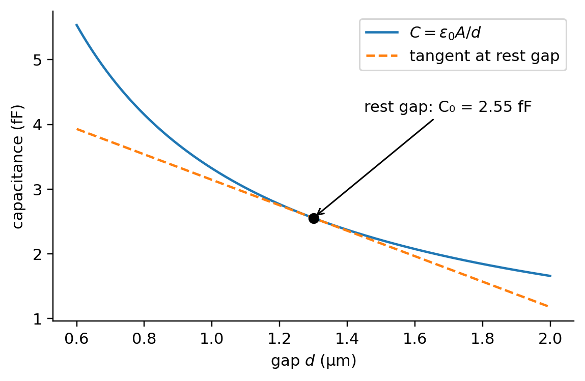

Figure 3.4: Capacitance of a single MEMS-scale finger pair (overlap 125 µm \(\times\) 3 µm, rest gap 1.3 µm) as the gap changes. The tangent at the rest gap is the local sensitivity; the departure from it is the nonlinearity a single-ended capacitive sensor would show.

3.4.3 Inductive

Reading the current in a live conductor without cutting it sounds impossible until magnetic coupling does the work for you. A current \(I_p\) in a wire creates a magnetic field around it; a coil of \(N\) turns wound on an iron ring around the wire links that field; and Faraday’s law of induction says a changing field induces a current in the coil. For an ideal transformer the induced secondary current is

\[ I_s = \frac{I_p}{N}, \tag{3.4}\]

so a 3000-turn CT turns 75 A into 25 mA. Pass that through a burden resistor \(R_b\) and you have a voltage, \(V = I_s R_b\), that a converter can read. Real CTs deviate slightly from Equation 3.4: the CR3110-3000’s sheet quotes an effective turns ratio of 3100 (including losses), a secondary resistance of 440 Ω, and a saturation voltage; it also tells you to keep \(V\) below 80% of the available voltage headroom for good linearity, so a 100 Ω burden gives 2.42 V at full current, comfortably inside the linear region.

The physics also sets the limits. Induction needs a changing field, so a CT cannot see direct current at all, and this one is rated from 20 Hz to 1 kHz. The same coupling principle, applied to a core that moves inside a pair of coils, gives the LVDT (linear variable differential transformer), the standard for precise, wear-free displacement measurement in structural testing, and eddy-current probes for non-contact proximity.

3.4.4 Piezoelectric

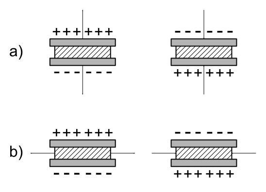
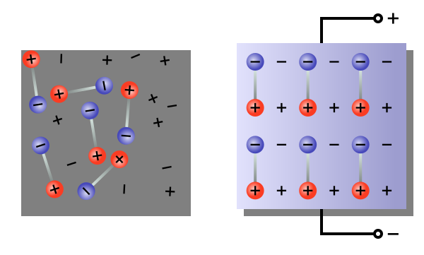
Measuring an impact or a vibration at kilohertz rates needs a sensor that generates its own signal, instantly, with no bridge and no supply. Certain crystals do exactly that (Figure 3.5). In quartz, and in ceramics whose internal dipoles have been permanently aligned, mechanical stress displaces charge within the lattice so that a charge \(Q\) appears across the faces, proportional to the applied force \(F\),

\[ Q = d\,F, \qquad V = \frac{Q}{C} = \frac{d\,F}{C}, \tag{3.5}\]

where \(d\) is the piezoelectric coefficient (about 2.3 pC/N for quartz) and \(C\) the capacitance of the crystal and its wiring. Ten newtons on a quartz element with 100 pF of total capacitance gives 23 pC and 0.23 V — small, but enormous compared with the nothing that a resistive element would produce without excitation.

Two consequences follow directly from Equation 3.5. Because the crystal produces charge only while stress changes, the charge leaks away through any finite resistance, and a piezoelectric sensor cannot hold a static reading: it is blind to DC and to very slow signals. And because the effect is a lattice property with no moving parts to speak of, it is extremely fast and stiff, with resonances in the tens of kilohertz. That combination — self-generating, fast, no DC — is the signature of the piezoelectric accelerometers used for experimental modal analysis of structures. The Wikipedia article on piezoelectricity goes further into the crystal physics.

(a) An X-cut piezoelectric plate: stretching or compressing it along either axis separates charge of opposite sign on the two faces, and the sign reverses with the direction of the force. (CLI, Wikimedia Commons, CC0.)

(b) Poling a ceramic: dipoles that are randomly oriented as manufactured (left) are aligned by a strong electric field above the Curie temperature and stay aligned once cooled (right), giving the ceramic a net piezoelectric response. (wdwd, Wikimedia Commons, CC BY-SA 3.0.)

Figure 3.5: The direct piezoelectric effect in a crystal plate, and the poling that creates it in a ceramic.

3.4.5 Thermoelectric

Some temperatures — inside a furnace, on rebar during a fire test — are beyond what a thermistor survives. A junction of two dissimilar metals produces a voltage that depends on the temperature difference between it and a second, reference junction: the Seebeck effect. The thermocouple built on it is passive, rugged, cheap, and covers ranges of well over a thousand degrees; the price is a small signal (tens of microvolts per degree), a nonlinear relation, and the fact that it only ever measures a difference, so the reference junction’s temperature must be known — the cold-junction compensation that every thermocouple readout performs, usually with a thermistor. This is the relative sensor of Section 3.3.2.

3.4.6 Optical

Copper wires pick up electrical noise and corrode, which matters when you instrument a dam or a bridge deck for decades. Optical sensors modulate light instead — its intensity, phase, wavelength, or time of flight — and light does not care about electromagnetic interference or moisture. The fiber Bragg grating (Wikipedia) is the structural engineer’s example: a periodic pattern written into an optical fiber reflects one specific wavelength, and stretching the fiber changes the pattern’s period and therefore the reflected color, so strain and temperature are read as a wavelength shift. Dozens of gratings can sit on one fiber. LiDAR measures distance by time of flight, turbidity meters measure water quality by scattered intensity, and the humble photoresistor measures light level — though, as noted, its readout is resistive.

3.4.7 One Measurand, Three Principles: The Accelerometer

The accelerometer breaks our neat one-principle-per-sensor picture, and the way it breaks it is the most useful idea in this section. You can buy piezoelectric accelerometers, piezoresistive ones, and capacitive ones. How can three different physical effects all measure the same thing?

The answer is that none of them measures acceleration directly. Every accelerometer is a complex sensor in Fraden’s sense: a mechanical front end followed by a displacement transducer. The front end is a seismic mass \(m\) attached to the case through a spring of stiffness \(k\) and a damper \(c\) (Figure 3.6). When the case accelerates with \(\ddot x\), the mass lags behind, and its displacement \(z\) relative to the case obeys

\[ m\,\ddot z + c\,\dot z + k\,z = -m\,\ddot x . \tag{3.6}\]

For slow enough motion the inertia and damping terms are negligible and \(z \approx -(m/k)\,\ddot x\): the relative displacement is simply proportional to the acceleration. The job of the second stage is to read \(z\), and any displacement transducer will do:

• a piezoelectric element, squeezed by the mass, producing charge (fast, high resonance, no DC — the modal-analysis instrument);
• a piezoresistive element, a semiconductor strain gauge on the flexure holding the mass (responds down to DC, good for slowly varying loads);
• a capacitive element, the mass carrying one set of plates (the ADXL335 and every MEMS accelerometer in a phone: down to DC, low power, tiny).

So the datasheet difference between a laboratory piezoelectric accelerometer for modal testing and an ADXL335 is not in the front end but in the readout — and, as Section 3.7 will show, the front end’s own dynamics in Equation 3.6 set the usable frequency range of all three.

fig, ax = plt.subplots(figsize=(5.2, 3.4)); ax.set_aspect("equal"); ax.axis("off")
ax.plot([0, 0, 6, 6], [4, 0, 0, 4], color="k", lw=2)                       # case
ax.fill_between([-.5, 6.5], -.8, 0, color="0.8", hatch="///", edgecolor="0.5", lw=0)
ax.text(3, -1.75, "structure surface (moves with x)", ha="center", fontsize=8)
ys = np.linspace(0, 2.2, 12)                                                # spring
xs = 1.6 + 0.25 * np.where(np.arange(12) % 2 == 0, 1, -1); xs[0] = xs[-1] = 1.6
ax.plot(xs, ys, color="k"); ax.text(0.7, 1.1, "k", fontsize=12)
ax.plot([4.4, 4.4], [0, 0.9], color="k"); ax.plot([4.1, 4.7], [0.9, 0.9], color="k")   # damper
ax.plot([4.05, 4.05, 4.75, 4.75], [1.5, 0.75, 0.75, 1.5], color="k"); ax.plot([4.4, 4.4], [1.5, 2.2], color="k")
ax.text(5.05, 1.1, "c", fontsize=12)
ax.add_patch(plt.Rectangle((1.2, 2.2), 3.6, 1.0, facecolor="#9ecae1", edgecolor="k"))   # mass
ax.text(3, 2.7, "seismic mass  m", ha="center", va="center", fontsize=10)
ax.add_patch(plt.Rectangle((2.75, 0.2), 0.5, 2.0, facecolor="#fdd0a2", edgecolor="k"))  # transducer
ax.annotate("displacement transducer", (3.0, 0.25), xytext=(3.0, -1.2), ha="center", fontsize=8, arrowprops=dict(arrowstyle="->", color="0.3"))
ax.annotate("", (6.6, 1.2), (6.6, 0.0), arrowprops=dict(arrowstyle="<->")); ax.text(6.75, 0.5, "x (case)", fontsize=9)
ax.annotate("", (5.6, 3.4), (5.6, 2.2), arrowprops=dict(arrowstyle="<->")); ax.text(5.75, 2.7, "z (relative)", fontsize=9)
ax.set_xlim(-0.6, 8.2); ax.set_ylim(-2.0, 3.8)
plt.show()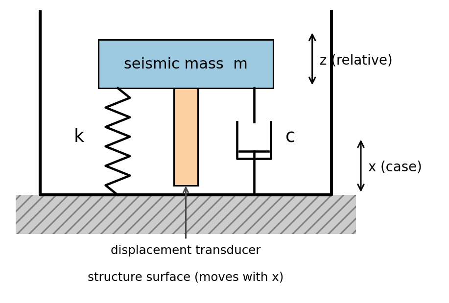

Figure 3.6: The seismic-mass model behind every accelerometer: a mass on a spring and damper inside a case that moves with the structure. The displacement transducer (piezoelectric, piezoresistive, or capacitive) reads the relative displacement z.

Table 3.2: The six transduction principles at a glance.

Principle	Governing relation	What changes	Passive / active	Canonical CEE sensor	Typical measurand
Resistive	\(R = \rho\,l/a\); \(R = R_0[1+\alpha\Delta T]\)	resistance	active	foil strain gauge; RTD/thermistor; photoresistor	strain; temperature; light
Capacitive	\(C = \varepsilon_0\varepsilon_r A/d\)	capacitance	active	MEMS accelerometer; polymer humidity sensor	acceleration; humidity; level
Inductive	\(I_s = I_p/N\) (Faraday)	current / inductance	passive (CT), active (LVDT)	split-core CT; LVDT	AC current; displacement
Piezoelectric	\(Q = d\,F\)	charge	passive	piezo accelerometer; dynamic force sensor	vibration; impact; dynamic pressure
Thermoelectric	Seebeck voltage \(\propto \Delta T\)	voltage	passive	thermocouple	high / wide-range temperature
Optical	e.g. Bragg wavelength shift	light intensity / wavelength / time of flight	active (needs a source)	fiber Bragg grating; LiDAR; turbidity meter	strain; distance; water quality

TipActive Learning: Classify Six Sensors

Six sensors, four of which you have only seen mentioned so far — here is what each one is, in a line:

• Thermocouple — two wires of different metals welded together at the tip; the voltage between the free ends depends on the tip temperature (background; NIST reference tables).
• Pt100 RTD — a thin platinum resistor trimmed to exactly 100 Ω at 0 °C (background; Vishay PTS datasheet).
• LVDT — a movable iron core sliding inside a primary coil and two secondary coils; the core’s position sets how the AC excitation couples into each secondary (how it works; background).
• DHT11 — a hobbyist temperature-and-humidity module: a capacitive humidity element and a thermistor read by a tiny microcontroller that outputs digital values (datasheet).
• Laboratory piezoelectric accelerometer — e.g. the PCB 352C33: a ceramic shear element under a seismic mass, with built-in electronics that convert charge to voltage (spec sheet).
• Fiber Bragg grating strain sensor — e.g. the Luna os3100: an FBG held in tension in a steel carrier that is welded or glued to the structure (product page).

Now, before opening the links, classify each along both axes — device kind (passive/active, absolute/relative, from Section 3.3.2) and transduction principle (from Table 3.2). Then open each datasheet and check your answers against what it says about excitation and output. One of the six is a trap: its transducer is passive, but the electronics packaged with it need a supply — decide how you want to classify that.

CautionConcept Check: Which one needs an excitation source?

Recall the two temperature sensors of Section 3.4: a thermocouple is a junction of two dissimilar metals that produces a Seebeck voltage, and an RTD is a platinum resistor whose resistance follows Equation 3.2. Both measure temperature. Which of them needs an excitation source to produce an output, and what does that tell you about the physics each relies on?

TipAnswer

The RTD. Its output is a resistance, and a resistance is not a signal until you pass a current through it — it is an active (parametric) sensor built on Equation 3.2. The thermocouple generates a voltage from the Seebeck effect with no supply at all — it is passive. The general rule: sensors whose governing relation ends in a resistance, capacitance, or inductance need excitation; those whose relation ends in a charge or a voltage do not.

3.5 Reading a Datasheet: Static Characteristics

Open the ADXL335 and CR3110-3000 sheets you found in Section 3.3.3. Between them they use every term in this section’s learning objective — sensitivity, range, resolution, nonlinearity, hysteresis, drift — plus accuracy and repeatability, and they use them in slightly different ways, because each manufacturer decides how to present its own numbers. Choosing the CT for a submetering job, or the accelerometer for a footbridge, is impossible without knowing what those numbers promise and, just as important, what they leave out. The key to reading any datasheet is that all of its numbers describe one object.

3.5.1 The Transfer Function

That object is the transfer function: the relation between the stimulus \(s\) and the sensor’s electrical response \(S\),

\[ S = f(s), \tag{3.7}\]

in Fraden’s notation (Fraden 2016, Ch. 2). For an ideal sensor, \(f\) is a known curve — a formula from the physics, a calibration table, or a fitted polynomial — and if you know \(f\) you can invert it to recover the stimulus from what you measured: \(s = f^{-1}(S)\). In practice we usually want \(f\) to be a straight line,

\[ S = S_0 + B\,(s - s_0), \tag{3.8}\]

because a line has only two parameters, needs only two calibration points, and inverts trivially. Most of the datasheet is then either a property of that line or a bound on how far the real sensor strays from it. Figure 3.7 puts every term of this section on one picture; the subsections that follow just walk around it.

s = np.linspace(0, 10, 400)
B, S0 = 10.0, 0.0                                  # ideal: 10 mV per mm
ideal = S0 + B * s
bend = 22.0 * np.sin(np.pi * s / 10)               # nonlinearity, exaggerated to be legible
loop = 9.0 * np.sin(np.pi * s / 10)                # half-width of the hysteresis loop, exaggerated
real_up = ideal + bend - loop                      # loading sweep
real_dn = ideal + bend + loop                      # unloading sweep
drift = ideal + 16.0
fig, ax = plt.subplots(figsize=(6.8, 4.8))
ax.plot(s, ideal, "k--", lw=1.2, label="ideal line (slope = sensitivity $B$)")
ax.plot(s, real_up, color="C0", label="real curve, loading")
ax.plot(s, real_dn, color="C0", ls=":", label="real curve, unloading")
ax.plot(s, drift, color="C3", lw=1, alpha=0.7, label="same sensor after drift")
# nonlinearity: vertical gap between the ideal line and the mid-loop curve at s = 7
i7 = 280
ax.annotate("", (7, ideal[i7]), (7, ideal[i7] + bend[i7]), arrowprops=dict(arrowstyle="<->", color="C2"))
ax.text(7.2, ideal[i7] + bend[i7] / 2, "δ  nonlinearity", color="C2", fontsize=9, va="center")
# hysteresis: horizontal gap between loading and unloading at S = 35 mV
i_up = np.argmin(abs(real_up - 40)); i_dn = np.argmin(abs(real_dn - 40))
ax.annotate("", (s[i_up], 40), (s[i_dn], 40), arrowprops=dict(arrowstyle="<->", color="C1"))
ax.text((s[i_up] + s[i_dn]) / 2, 31, "h  hysteresis", color="C1", ha="center", fontsize=9)
# range
ax.axvline(0, color="0.6", lw=0.8); ax.axvline(10, color="0.6", lw=0.8)
ax.annotate("", (0, 136), (10, 136), arrowprops=dict(arrowstyle="<->", color="0.4"))
ax.text(5, 138, "range (span, full scale)", ha="center", fontsize=9, color="0.3")
# resolution: staircase near the origin
ss = np.linspace(0, 1.2, 200); ax.step(ss, np.floor(B * ss / 2) * 2, where="post", color="C4", lw=1)
ax.text(1.35, 3, "resolution\n(smallest step)", color="C4", fontsize=8, va="center")
ax.annotate("drift", (8.5, drift[340]), xytext=(6.2, 124), color="C3", fontsize=9, arrowprops=dict(arrowstyle="->", color="C3"))
ax.set_xlabel("stimulus $s$ (mm)"); ax.set_ylabel("output $S$ (mV)"); ax.set_xlim(-0.3, 10.8); ax.set_ylim(-3, 144)
ax.legend(loc="lower right", fontsize=8)
plt.show()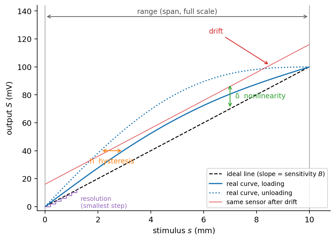

Figure 3.7: One transfer function carrying every static characteristic (departures exaggerated for legibility): the ideal line and its slope (sensitivity) over the guaranteed span (range); a real curve that departs from the line (nonlinearity \(\delta\)), that differs between loading and unloading (hysteresis \(h\)), that is only resolved in finite steps (resolution), and that shifts as a whole with time or temperature (drift).

3.5.2 Sensitivity, Range, and Resolution

Before you buy a sensor you must answer three questions: how much output do I get per unit of input, over what span is that guaranteed, and how small a change can I actually see?

Sensitivity is the slope \(B\) of the transfer function — output per unit stimulus. The ADXL335 quotes 300 mV/g (typical) at a 3 V supply, with a guaranteed window of 270–330 mV/g, i.e. ±10% part-to-part. Read that tolerance twice: unless you calibrate each device, a 1 g reading could be off by 0.1 g from sensitivity alone, which as we will see dwarfs every other error on the sheet. The CT expresses the same idea as a ratio: 1 A of primary current gives 1/3100 A in the secondary, so with a 100 Ω burden the sensitivity is 32 mV/A. For nonlinear sensors the sensitivity is the local slope \(\mathrm{d}S/\mathrm{d}s\) and varies with the stimulus — the photoresistor’s resistance-versus-lux curve is one, which is why its sheet gives a gamma (the log-log slope between 10 and 100 lux) rather than a single number.

Range (span, or input full scale) is the stimulus interval over which the datasheet’s promises hold. The ADXL335 guarantees ±3 g; the CT senses up to 75 A linearly and tolerates four times that briefly. The corresponding output interval is the full-scale output (FSO): ±3 g × 300 mV/g = ±0.9 V about the 1.5 V zero-g level, i.e. 0.6–2.4 V, safely inside the 0–3 V supply rails. Push past the range and most sensors saturate — the output stops responding — which is what the CT’s “maximum voltage” specification is warning about.

Resolution is the smallest change in stimulus that produces a distinguishable change in output. For a digital sensor it is set by the number of bits; for an analog one it is usually set by noise. The ADXL335 does not quote a resolution directly; it quotes a noise density, 150 µg/√Hz on the X and Y axes, from which the resolution follows once you decide the bandwidth: over 100 Hz, \(150\ \mu\text{g}\times\sqrt{1.6 \times 100\ \text{Hz}} \approx 1.9\) mg rms (the factor 1.6 accounts for the filter’s shape). Lecture 4 will revisit this from the converter’s side.

3.5.3 Accuracy and Repeatability

A sensor that reports six decimal places can still be wrong by a full percent, and a sensor that is always wrong by the same amount is more useful than one that is right on average but scatters. These two sentences are the whole content of the most-confused pair of terms on any datasheet.

Accuracy (Fraden points out it really means inaccuracy) is the largest deviation between the value a sensor reports and the true value of the stimulus, including every contributing error: calibration, nonlinearity, hysteresis, drift, part-to-part variation. It is quoted in the units of the stimulus (±0.5 °C), as a percentage of full scale (±2% FS), or as a percentage of the reading. Many sheets — the ADXL335’s among them — never quote a single accuracy number at all; they quote the components and leave the combination to you.

Repeatability is the spread of outputs for repeated, identical stimuli under identical conditions — the width of the cloud, not its distance from the truth. It is a component of accuracy but is often quoted separately because it is the one error you cannot calibrate away: a systematic offset can be measured and subtracted, random scatter cannot. And resolution, from the previous subsection, is a third, independent quantity: the granularity of the output says nothing about whether the value is right. A digital scale reading to 0.01 g can be repeatable to 0.01 g and inaccurate by 5 g if it was calibrated with the wrong reference weight.

CautionConcept Check: Which sensor do you choose?

Three displacement sensors are on offer for monitoring the slow settlement of a foundation over a year. Sensor A resolves 1 µm but its readings scatter by ±50 µm when the same displacement is repeated. Sensor B resolves only 20 µm but repeats to ±20 µm and is accurate to ±30 µm. Sensor C resolves 5 µm, repeats to ±5 µm, and is accurate to ±200 µm because its factory calibration is poor. Which do you choose, and why does the one with the most decimal places not win?

TipAnswer

Sensor C, provided you calibrate it yourself once against a reference — its poor accuracy is a systematic error, which one calibration removes, leaving ±5 µm repeatability. Sensor A’s fine resolution is useless because its ±50 µm scatter is random and cannot be removed. Sensor B is the safe choice if you cannot calibrate. Resolution tells you the granularity of the number, repeatability tells you how much of it is noise, accuracy tells you how far it may be from the truth — and only the middle one is beyond your control.

3.5.4 Linearity, Hysteresis, and Drift

The catalog assumes the ideal line of Equation 3.8, but your bridge sensor returns different readings on the way up and on the way down, and different readings in July than in January. Three numbers on the datasheet bound those departures.

Nonlinearity is the maximum deviation of the real transfer function from the straight line used to approximate it, usually quoted as a percentage of full scale. The ADXL335 claims ±0.3% FS, which on a 6 g span is 18 mg. Beware that the number depends on which line: through the end points, the best-fit line, or a line tangent at a calibration point can give quite different nonlinearity figures for the same sensor, and a manufacturer will naturally publish the smallest. If the sheet does not say which line, the number is not fully meaningful.

Hysteresis is the difference in output at the same stimulus depending on the direction from which it was approached — the loop between the loading and unloading curves in Figure 3.7. Friction, mechanical play, and material memory cause it; it is common in anything with a moving part or a polymer in it, and it is usually quoted as a percentage of full scale.

Drift is the slow change of the transfer function with time or with an environmental variable, most often temperature. Short-term drift over minutes to days is effectively a form of repeatability error; long-term drift over months is aging and is usually one-directional. Temperature drift is quoted per degree: the ADXL335 lists a zero-g offset drift of ±1 mg/°C and a sensitivity drift of ±0.01%/°C. Over a 25 °C swing, the offset alone moves 25 mg — more than the nonlinearity.

Putting these together into a statement about one reading is the business of Lecture 7, but you can already see the shape of it: at 1 g on an uncalibrated ADXL335, the sensitivity tolerance contributes up to 100 mg, the nonlinearity 18 mg, and a 25 °C temperature excursion 25 mg. The lesson generalizes far beyond this part: the biggest error term is usually the one that calibration would remove, which is why instruments get calibrated.

Figure 3.8 does the datasheet’s job in reverse: given a calibration sweep of a fictional displacement sensor — up and down, repeated — it extracts the sensitivity, the nonlinearity, the hysteresis, and the repeatability, exactly as a manufacturer’s test bench would.

rng = np.random.default_rng(12778)
s_pts = np.linspace(0, 10, 11)
B_true, hyst_true, noise = 10.0, 1.0, 0.3         # mV/mm, mm, mV (departures exaggerated for legibility)
def true_curve(s, direction):                     # direction: +1 loading, -1 unloading
    return B_true * s + 7.0 * np.sin(np.pi * s / 10) - direction * B_true * hyst_true / 2 * np.sin(np.pi * s / 10) ** 0.5
runs_up = np.array([true_curve(s_pts, +1) + rng.normal(0, noise, s_pts.size) for _ in range(3)])
runs_dn = np.array([true_curve(s_pts, -1) + rng.normal(0, noise, s_pts.size) for _ in range(3)])
S_all = np.concatenate([runs_up, runs_dn]); s_all = np.tile(s_pts, 6)
B_fit, A_fit = np.polyfit(s_all, S_all.ravel(), 1)
fs_out = B_fit * 10
nonlin = np.max(np.abs(S_all.mean(axis=0) - (A_fit + B_fit * s_pts))) / fs_out * 100        # % FSO
hyst_mV = np.max(np.abs(runs_dn.mean(axis=0) - runs_up.mean(axis=0)))
repeat = max(runs_up.std(axis=0, ddof=1).max(), runs_dn.std(axis=0, ddof=1).max())
fig, ax = plt.subplots(figsize=(6.2, 4))
for r in runs_up: ax.plot(s_pts, r, "o", color="C0", ms=3, alpha=0.6)
for r in runs_dn: ax.plot(s_pts, r, "s", color="C1", ms=3, alpha=0.6)
ax.plot(s_pts, runs_up.mean(axis=0), color="C0", label="loading (mean of 3)")
ax.plot(s_pts, runs_dn.mean(axis=0), color="C1", label="unloading (mean of 3)")
ax.plot(s_pts, A_fit + B_fit * s_pts, "k--", label=f"best fit: {B_fit:.2f} mV/mm")
ax.set_xlabel("displacement (mm)"); ax.set_ylabel("output (mV)"); ax.legend()
ax.set_title(f"nonlinearity {nonlin:.1f}% FSO · hysteresis {hyst_mV/B_fit:.2f} mm · repeatability ±{repeat/B_fit*1e3:.0f} µm (1σ)", fontsize=9)
plt.show()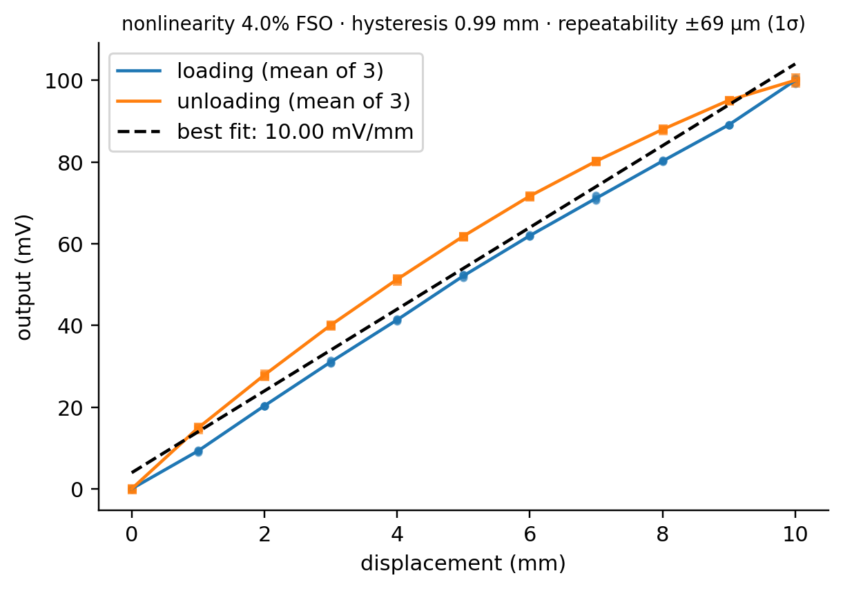

Figure 3.8: A synthetic calibration record for a displacement sensor (nominal 10 mV/mm, 0–10 mm; departures exaggerated for legibility): three loading/unloading cycles with noise. The best-fit line gives the sensitivity; the largest departure from it the nonlinearity; the loading–unloading gap the hysteresis; the scatter of repeated points the repeatability.

TipActive Learning: One Sheet, Three Jobs

Take the ADXL335 datasheet and decide, with numbers pulled from the sheet, whether the part can serve each of these three jobs: (a) detecting the ~2 Hz sway of a pedestrian bridge with ±10 mg amplitude; (b) measuring the tilt of a retaining wall to 0.1° (hint: tilt is a change in the static 1 g reading — how many mg is 0.1°?); (c) logging truck-induced vibration on a highway overpass at up to 500 Hz. For each, name the single characteristic that decides the answer. Then do the same for the CR3110-3000 with: (d) monitoring a 20 A single-phase circuit; (e) a 200 A service entrance; (f) a DC solar array.

3.6 Matching Sensors to CEE Measurands

Your final project will require picking real sensors for real measurands, and the catalog offers a dozen ways to measure any of them. But the previous three sections already gave you the filters. Sensor selection is a short sequence of questions, each of which points back to something you now know:

1. What quantity, exactly? Strain or displacement? Acceleration or tilt? Current or power? (Section 3.3 — name the measurand before the sensor.)
2. Static or dynamic? Do you need DC response (settlement, tilt, temperature) or only changes (vibration, impact)? This alone rules piezoelectric sensors in or out (Section 3.4).
3. What range and resolution? Full scale with margin, and the smallest change that matters — read against the sheet’s sensitivity, span, and noise (Section 3.5).
4. What environment? Temperature swings (drift), moisture and corrosion (optical wins), electromagnetic interference (optical again), access for recalibration.
5. What installation, power, and budget? Passive or active, wired or wireless, how many channels, and what data-acquisition system it must talk to (Lecture 4). ### Modalities by Application Domain

Project teams think in terms of a system to instrument rather than a list of measurands, so Table 3.3 is organized the way you will use it. Each cell names the two or three modalities that dominate practice, by the principle we have studied, and why they won.

Table 3.3: Dominant sensing modalities by application domain.

Domain	Measurand	Dominant modalities (principle)	Why they won
Structural health monitoring	strain	foil strain gauge (resistive); fiber Bragg grating (optical)	gauges are cheap and well understood; FBGs multiplex on one fiber and ignore EMI for long-term deployments
	displacement	LVDT (inductive); laser/optical; GNSS at bridge scale	LVDT is wear-free and precise; optical for non-contact
	acceleration	MEMS capacitive (e.g. ADXL335) for ambient vibration; piezoelectric for modal testing	MEMS: DC-capable, cheap, low power; piezo: high bandwidth, self-generating
Building energy	temperature	thermistor / RTD (resistive); thermocouple for extremes	thermistors are cheap and sensitive; RTDs stable; thermocouples rugged
	humidity	capacitive polymer sensor	low power, adequate accuracy, integrates with temperature on one chip
	electrical current / power	split-core CT (inductive); Hall-effect for DC	CTs clamp on without rewiring; Hall sensors see DC
Transportation	vehicle presence / count	inductive loop; piezoelectric strip; camera / LiDAR (optical)	loops are embedded and durable; piezo strips give axle timing; optical adds classification
	pavement / bridge response	strain gauge, accelerometer (as above)	—
Water (brief)	flow	electromagnetic, ultrasonic, differential pressure	no moving parts (EM, ultrasonic) or simplicity (ΔP)
	water quality	electrochemical probes (pH, DO); optical turbidity	each parameter has its own dedicated chemistry or optics

ImportantExercise: A Pedestrian Bridge Campaign

A 60 m steel pedestrian bridge is to be monitored for one year to characterize pedestrian-induced vibration (expected 1–3 Hz, up to 0.1 g), thermal expansion at the bearings (±15 mm over the year), and strain at two welded connections. The budget is modest, mains power is available at one abutment only, and the deck is exposed to weather. Specify a sensor for each of the three measurands and justify each choice against the five selection questions.

TipOne defensible answer

Vibration: a MEMS capacitive accelerometer (ADXL335-class or a digital successor): the 1–3 Hz, 0.1 g signal is well inside its range and bandwidth, it responds down to DC so the mounting orientation can be checked, and it runs on milliwatts — decisive given power is only available at one end. A piezoelectric accelerometer would need a powered charge amplifier and offers bandwidth you do not need. Bearing displacement: an LVDT or a draw-wire potentiometer: ±15 mm is a large, slow, DC displacement, which rules out anything piezoelectric and favors a robust contact sensor; both need excitation, so run them from the powered abutment. Strain: foil strain gauges in a bridge configuration are the budget answer, with temperature-compensating dummy gauges since the deck is exposed; if the budget stretched and EMI or long cable runs were a concern, FBGs on a single fiber would be the premium choice.

3.7 How Transducer Physics Shapes Your Data

An anomaly detector once flagged a “sudden” temperature spike in a plant room that never happened. The probe had lagged behind a real, slow change and then caught up; the model, trained on the recorded values, learned the sensor rather than the room. Nothing in the data said so. This section is about the ways the physics that makes a transducer work also limits it — its own dynamics, its interaction with the thing measured, and its response to stimuli you never meant to measure — and about why those limits reappear downstream as artifacts a model will cheerfully fit.

3.7.1 Dynamics and Bandwidth

Everything in Section 3.5 quietly assumed the stimulus held still — that is why those characteristics are called static. Drop a thermometer into hot water and it does not read the true temperature instantly, because heat must flow into it first. The accelerometer’s seismic mass, likewise, cannot follow a vibration faster than its own spring lets it. When the stimulus varies in time, the sensor’s response generally does not follow with perfect fidelity, and the difference is the dynamic error.

Fraden classifies sensors by the order of the differential equation that links output to input. A zero-order sensor responds instantly (a potentiometer, near enough). A first-order sensor has one energy store — the heat capacity of a thermometer — and obeys

\[ \tau\,\frac{\mathrm{d}y}{\mathrm{d}t} + y = x, \tag{3.9}\]

where \(x\) is the true stimulus, \(y\) the reading, and \(\tau\) the time constant. After a step change in \(x\), the reading covers 63.2% of the change at \(t = \tau\) and 95% at \(t = 3\tau\); equivalently, the sensor attenuates sinusoidal stimuli above a cutoff frequency \(f_c \approx 0.159/\tau\). A DHT11 humidity module quotes a 6 s response time in moving air; a sheathed thermocouple in still air can have \(\tau\) of tens of seconds. Figure 3.9 is the plant-room story from the opening of this section, simulated: the same first-order probe following a step and a slow ramp, and a naive detector misreading the lag.

from scipy.integrate import solve_ivp
tau = 30.0
t = np.linspace(0, 600, 1201)
x_step = np.where(t >= 60, 1.0, 0.0)
x_ramp = np.clip((t - 60) * (2.0 / 300), 0, 2.0)
def respond(x_fun):
    sol = solve_ivp(lambda tt, y: (np.interp(tt, t, x_fun) - y) / tau, [0, 600], [0.0], t_eval=t, max_step=0.5)
    return sol.y[0]
y_step, y_ramp = respond(x_step), respond(x_ramp)
lag_ss = tau * (2.0 / 300)
fig, axs = plt.subplots(3, 1, figsize=(6.4, 6.2), sharex=True)
axs[0].plot(t, x_step, "k", label="true (step)"); axs[0].plot(t, y_step, "C0", label="reading")
axs[0].axvline(60 + tau, color="0.7", ls=":"); axs[0].text(60 + tau + 3, 0.2, "t = τ: 63%", fontsize=8)
axs[0].set_ylabel("°C above start"); axs[0].legend(loc="lower right", fontsize=8)
axs[1].plot(t, x_ramp, "k", label="true (ramp)"); axs[1].plot(t, y_ramp, "C0", label="reading")
axs[1].annotate("", (200, x_ramp[400]), (200, y_ramp[400]), arrowprops=dict(arrowstyle="<->", color="C3"))
axs[1].text(212, y_ramp[400] - 0.12, f"lag = τ·slope = {lag_ss:.2f} °C", color="C3", fontsize=8, va="top")
axs[1].set_ylabel("°C above start"); axs[1].legend(loc="lower right", fontsize=8)
rate_true = np.gradient(x_ramp, t) * 60; rate_read = np.gradient(y_ramp, t) * 60
thr = 0.2   # °C per minute
axs[2].fill_between(t, 0, 1, where=rate_true > thr, color="k", alpha=0.15, label="true rate > 0.2 °C/min")
axs[2].fill_between(t, 0, 1, where=rate_read > thr, color="C3", alpha=0.35, label="detector on reading")
axs[2].set_yticks([]); axs[2].set_xlabel("time (s)"); axs[2].legend(loc="upper right", fontsize=8)
plt.tight_layout(); plt.show()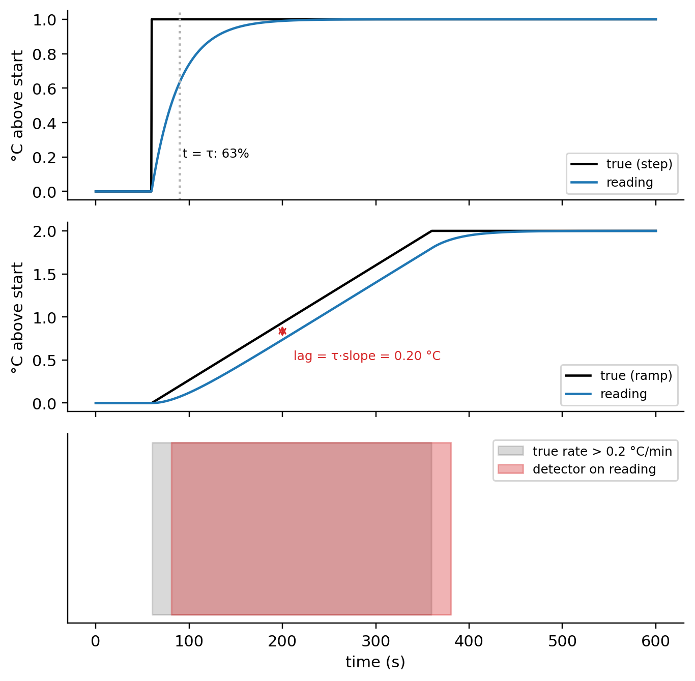

Figure 3.9: A first-order temperature probe (\(\tau\) = 30 s) following a step and a 2 °C ramp over 5 minutes. During the ramp the reading lags the truth by a constant \(\tau \times\) slope = 0.2 °C; after the ramp ends it keeps rising for about \(3\tau\). A detector thresholding the reading’s rate of change (bottom) turns on and off about \(\tau \ln 2 \approx 21\) s late — it is detecting the sensor, not the room.

Move the slider to see how the lag scales with the time constant; the ramp is the same 2 °C over 5 minutes.

viewof tauW = Inputs.range([5, 120], {value: 30, step: 5, label: "time constant τ (s)"})

lagSeries = {
  const T = 300, a = 2 / T, t0 = 60, rows = [];
  const yEnd = a * (T - tauW * (1 - Math.exp(-T / tauW)));
  for (let t = 0; t <= 600; t += 2) {
    const u = t - t0;
    const x = u < 0 ? 0 : (u < T ? a * u : 2);
    const y = u < 0 ? 0 : (u < T ? a * (u - tauW * (1 - Math.exp(-u / tauW))) : 2 - (2 - yEnd) * Math.exp(-(u - T) / tauW));
    rows.push({t, series: "true temperature", value: x});
    rows.push({t, series: "probe reading", value: y});
  }
  return rows;
}
Plot.plot({
  height: 260, marginLeft: 50,
  x: {label: "time (s)"}, y: {label: "°C above start", domain: [0, 2.2]},
  color: {legend: true, domain: ["true temperature", "probe reading"], range: ["black", "steelblue"]},
  marks: [Plot.line(lagSeries, {x: "t", y: "value", stroke: "series"}),
          Plot.text([{x: 590, y: 0.15, label: `steady-state lag ≈ ${(tauW * 2 / 300).toFixed(2)} °C`}], {x: "x", y: "y", text: "label", textAnchor: "end"})]
})

A second-order sensor has two energy stores — the mass and the spring of Equation 3.6 — and adds a resonance: a frequency \(f_n = \frac{1}{2\pi}\sqrt{k/m}\) near which the response is amplified rather than attenuated, by roughly \(1/(2\zeta)\) for damping ratio \(\zeta\). Below about 20% of \(f_n\) the response is flat to within a few percent — that is the usable band in which \(z \propto \ddot x\) holds — and above \(f_n\) it rolls off steeply. Figure 3.10 shows the shape; the derivation belongs to Lecture 6, but the consequence is immediate. A laboratory piezoelectric accelerometer for modal testing typically resonates above 30 kHz, giving a flat band to several kilohertz; a MEMS part resonates in the low kilohertz, and the ADXL335 additionally lets you choose its bandwidth with an external capacitor, \(f = 1/(2\pi \cdot 32\ \text{k}\Omega \cdot C)\) — 1.6 kHz with 3 nF, 500 Hz with 10 nF, and 0.5 Hz with 10 µF. Set 0.5 Hz because you only care about tilt, and the bridge vibration in your data simply vanishes — not because it stopped, but because you told the sensor not to see it. And on the other edge: the piezoelectric sensor’s blindness to DC (Section 3.4) is a lower cutoff of the same band.

r = np.logspace(-2, 1, 500)                      # f / f_n
fig, ax = plt.subplots(figsize=(6.2, 3.8))
for zeta in (0.05, 0.3, 0.7):
    H = 1 / np.sqrt((1 - r**2) ** 2 + (2 * zeta * r) ** 2)
    ax.loglog(r, H, label=f"ζ = {zeta}")
ax.axvspan(1e-2, 0.2, color="C2", alpha=0.12); ax.text(0.03, 0.55, "usable band\n(flat within ~4%)", fontsize=8, color="C2")
ax.axvline(1, color="0.6", ls=":"); ax.text(1.05, 0.25, "resonance $f_n$", fontsize=8, color="0.4")
ax.set_xlabel("frequency / resonant frequency"); ax.set_ylabel("normalized response"); ax.legend(); ax.set_ylim(0.05, 20)
plt.show()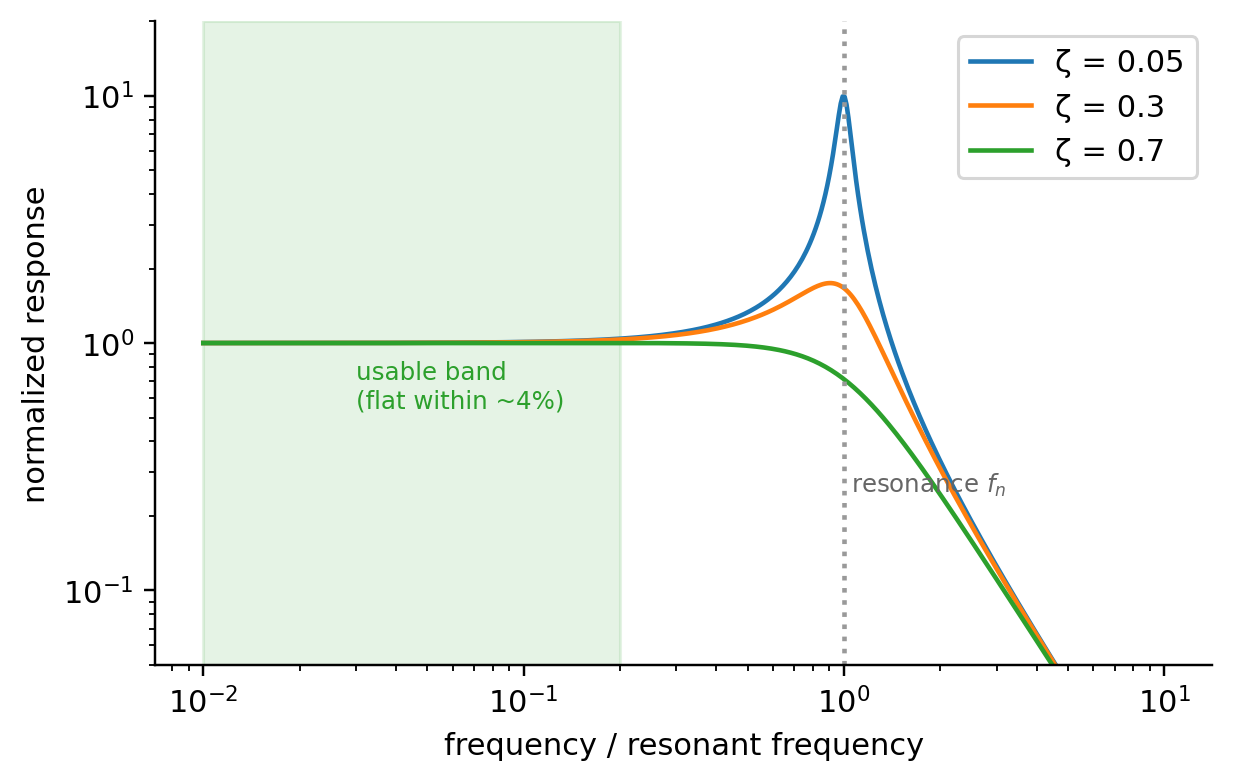

Figure 3.10: Magnitude of the seismic-mass response (relative displacement per unit base acceleration, normalized to its low-frequency value) for three damping ratios. The flat region is the usable band; the resonance amplifies by about \(1/(2\zeta)\); above it the sensor rolls off. Presented, not derived — see Lecture 6.

3.7.2 Loading and Cross-Sensitivity

A heavy accelerometer bolted to a light beam changes how the beam vibrates. A flow meter inserted in a pipe changes the flow it is there to measure. A thermocouple wicks heat away from the point whose temperature it reports. Attaching a sensor always changes the system, an effect called loading, and the honest question is never “does it?” but “by how much?” — a 10 g MEMS board on a bridge girder, not at all; a 100 g piezoelectric accelerometer on a laboratory-scale model, possibly a great deal. Active sensors add a loading of their own: the excitation current that a thermistor needs also heats it, so a thermistor in still air reads its own self-heating on top of the air temperature, which is why datasheets specify a maximum excitation current in air separately from that in water.

Most transducers also answer to more than one stimulus, which is called cross-sensitivity. The strain gauge’s resistance follows Equation 3.1 and Equation 3.2 at the same time, so a gauge on a steel beam in the sun reads thermal expansion and the resistivity change of its own foil as if they were strain — the reason strain-gauge installations carry temperature-compensating dummy gauges. The GL5528’s resistance depends on temperature as well as light. The ADXL335’s sheet quotes a ±1% cross-axis sensitivity (a Y acceleration leaking into the X output) and the temperature drifts we met in Section 3.5. And the current transformer’s cross-sensitivity is a blind spot rather than a leak: it cannot see DC, and it attenuates harmonics above 1 kHz, so a distorted waveform is reported as smoother and smaller than it is. The honest transfer function is therefore

\[ S = f(s, T, \ldots), \tag{3.10}\]

a function of the stimulus and of the environment, and a datasheet is largely a list of the partial derivatives with respect to the variables you did not intend to measure.

3.7.3 Consequences for Data and Models

None of these effects announce themselves in a CSV file. A first-order lag looks like a slow event; a resonance looks like a strong signal at \(f_n\) that is really the sensor ringing; a cross-sensitivity looks like a genuine correlation between temperature and strain that a regression model will happily learn and a physicist will immediately distrust. And none of it can be undone after the fact without knowing the physics: you can deconvolve a lag only if you know \(\tau\), and you can separate thermal from mechanical strain only if you know the gauge’s temperature coefficient and its temperature.

This is the reason the course insists on understanding the chain before modeling. Lecture 7 will turn the datasheet bounds of Section 3.5 into a formal uncertainty on each reading; the DATA third will show how metadata — which sensor, which bandwidth setting, which calibration — is what lets a dataset be interpreted at all; and the MODELS third will repeatedly ask whether a pattern a model found is in the world or in the instrument. The three lenses of this lecture — the chain, the principle, the characteristics — are how you tell.

CautionConcept Check: Which accelerometer for a tilting wall?

Two accelerometers have identical sensitivity and range. One is piezoelectric, the other capacitive MEMS. Which do you mount on a retaining wall that is suspected of tilting slowly over months, and why?

TipAnswer

The capacitive MEMS device. A slow tilt is a change in the static component of gravity along the sensor’s axis — a DC signal — and a piezoelectric sensor cannot hold a static reading (Equation 3.5: charge appears only while stress changes, and leaks away). The MEMS part responds down to DC, so 0.1° of tilt shows up as a persistent shift of about 1.7 mg in the reading along a horizontal axis. The two sheets’ identical sensitivity and range say nothing about this; the transduction principle says everything.

3.8 Putting It All Together

An instrument is a transducer surrounded by a chain of supporting links. The transducer works by one of a handful of physical effects, and the effect predicts the device’s behavior — speed, power, DC response, environmental sensitivity — before you open its datasheet. The datasheet then describes the transfer function that the effect produces and bounds how far a real device strays from it. And those same physics set what the data downstream can and cannot show, through dynamics, loading, and cross-sensitivity that no later processing can fully remove. The next lectures follow the chain link by link — circuits, data acquisition, signal conditioning, frequency-domain analysis, uncertainty — and the DATA and MODELS thirds inherit exactly what the physics let through, no more.

3.9 Exercises

1. Pick an everyday instrument other than the ruler or scale used above, and describe how it was designed, how it could be calibrated, and at least three ways it could drift or fail.

TipSolution sketch

A tire pressure gauge: designed around a range of 0–60 psi (or 0–4 bar) and a resolution of 1 psi; a piston against a calibrated spring, or a strain-based element in digital models; calibrated at the factory against a reference pressure standard (a deadweight tester). Failure modes: spring fatigue (sensitivity drift), dirt in the piston (hysteresis and dead band), temperature (the spring’s stiffness and the gas law both change), and a leaking seal (an offset that grows during the reading). Each maps onto a term in Section 3.5.

2. For the CR3110-3000 current transformer, draw its measurement chain from the current in the conductor to a number in a database, classify it along the axes of Section 3.3.2, and name its transduction principle.

TipSolution

Chain: alternating current in the conductor → alternating magnetic flux in the iron ring → induced current in the 3000-turn secondary (the sensor; inductive principle, Faraday’s law) → burden resistor converting current to voltage (signal conditioning) → anti-aliasing filter and analog-to-digital converter (signal processing, Lectures 4–5) → microcontroller computing an rms value and timestamping it → database row. Classification: passive (the energy comes from the measured circuit; no excitation), absolute (referenced to zero current), stimulus electric/magnetic, conversion phenomenon electromagnetic induction.

3. From the ADXL335 datasheet, extract sensitivity, range, resolution, accuracy, repeatability, nonlinearity, hysteresis, and drift, noting which are not given, and estimate the worst-case error on a 1 g reading (a) straight out of the box and (b) after a one-point gain calibration, over a 25 °C temperature swing.

TipSolution

Sensitivity 300 mV/g typical, 270–330 mV/g guaranteed (±10%) at 3 V; range ±3 g minimum; resolution not quoted directly — noise density 150 µg/√Hz on X/Y gives ≈1.9 mg rms over a 100 Hz bandwidth; accuracy not quoted as a single number; repeatability not quoted; nonlinearity ±0.3% FS = 18 mg on a 6 g span; hysteresis not quoted (the sheet mentions temperature hysteresis only qualitatively); drift: zero-g offset ±1 mg/°C, sensitivity ±0.01%/°C. Worst case at 1 g: (a) sensitivity tolerance 100 mg + nonlinearity 18 mg + offset drift 25 mg + sensitivity drift 0.25% × 1 g = 2.5 mg ≈ 146 mg; (b) with the ±10% gain error calibrated out, ≈ 46 mg, dominated by the temperature drift of the offset. The calibration removes two thirds of the error; the remaining term is the one that argues for a temperature sensor next to the accelerometer.

4. For a monitoring scenario of your choosing in one application domain of Table 3.3, specify a sensor for each of three measurands and justify each choice against the five selection questions of Section 3.6.

TipSolution sketch

Follow the pattern of the pedestrian-bridge exercise: for each measurand, state the quantity precisely, decide static vs. dynamic (which eliminates or admits piezoelectric devices), read range and resolution off a candidate datasheet, name the environmental threat (temperature, moisture, EMI) and the modality that handles it, and close with power and budget. A building-energy example: room temperature (thermistor; static; 10–35 °C to 0.1 °C; indoor; battery), supply-air humidity (capacitive polymer; slow; 20–90% RH to 3%; condensation risk — pick a sealed part), and circuit current (split-core CT; AC only; 0–75 A; clamp-on with no rewiring; passive).

5. A first-order temperature sensor with \(\tau = 30\) s records a room whose temperature ramps by 2 °C over 5 minutes and then holds. Sketch the recorded signal against the true one, state the lag during the ramp, and explain what a detector that flags “rate of change above 0.2 °C/min” would report.

TipSolution

During the ramp the reading approaches a constant lag of \(\tau \times\) slope \(= 30\ \text{s} \times (2\,^\circ\text{C}/300\ \text{s}) = 0.2\,^\circ\text{C}\) behind the truth (reached after a transient of about \(3\tau = 90\) s from the start of the ramp); after the ramp stops, the reading keeps rising and closes the gap over another \(\approx 3\tau\). The true rate of change is \(0.4\,^\circ\text{C}/\text{min}\) throughout the ramp and zero afterward. The detector on the reading turns on late — the recorded rate rises from zero with time constant \(\tau\) and crosses 0.2 °C/min at \(t = \tau \ln 2 \approx 21\) s after the ramp begins — and turns off late by the same \(\tau \ln 2\), since the recorded rate decays with the same time constant after the ramp ends. It reports an event that is shifted relative to the real one, and one that cannot be corrected without knowing \(\tau\) — exactly the artifact in Figure 3.9.

3.10 Additional Resources

• Datasheets used in this lecture: ADXL335 (Analog Devices), CR3100 series current transformers (CR Magnetics), GL55 series photoresistors.
• Wikipedia entries on the Seebeck effect, piezoelectricity, and fiber Bragg gratings for the physics we only sketched.

3.11 References

• Fraden (2016) (Chs. 1–4)
• Morris and Langari (2015) (Chs. 1–2)
• Figliola and Beasley (2019) (Chs. 1–2)

Figliola, Richard S., and Donald E. Beasley. 2019. Theory and Design for Mechanical Measurements. 7th ed. Wiley.

Fraden, Jacob. 2016. Handbook of Modern Sensors: Physics, Designs, and Applications. 5th ed. Springer.

Morris, Alan S., and Reza Langari. 2015. Measurement and Instrumentation: Theory and Application. 2nd ed. Academic Press.