Chapter setup: imports and shared names
import numpy as np
import matplotlib.pyplot as plt
import schemdraw
import schemdraw.elements as elmThis lecture assumes Lecture 2’s vocabulary — sensor, transducer, and the three electrical quantities (resistance, capacitance, inductance) that transduction principles end in — and nothing about circuits beyond high-school physics. Comfort with derivatives and integrals is expected; complex numbers make a brief appearance later and are reviewed when they do.
Every code block in this chapter assumes that the setup below has run first, in the same Python session: it imports the libraries and defines the names the blocks share (see About the code in the Welcome chapter).
import numpy as np
import matplotlib.pyplot as plt
import schemdraw
import schemdraw.elements as elmLecture 2 ended with the picture of an instrument as a transducer surrounded by supporting components, and quietly assumed that everything after the transducer is electrical. That was not inevitable: a bathroom scale worked perfectly well with a spring and a dial, and for decades industry ran on pneumatic instruments in which a measurement traveled as air pressure in a tube. Pneumatic and hydraulic measurement systems are the steam-punk alternatives that could have won — and they lost for concrete reasons (Putten 1988):
So it is no surprise that virtually every modern instrument is electronic, and the consequence is worth stating plainly: understanding a modern instrument is understanding circuit theory — the basic laws that govern how DC and AC circuits behave, and how they transform the signals passing through them.
But where does circuit theory itself come from? It is a limiting case of electromagnetism, the physics whose modern form we owe to James Clerk Maxwell.
You may have seen Maxwell’s celebrated equations:
\[ \nabla \cdot \mathbf{E} = \frac{\rho}{\varepsilon_0}, \qquad \nabla \cdot \mathbf{B} = 0, \qquad \nabla \times \mathbf{E} = -\frac{\partial \mathbf{B}}{\partial t}, \qquad \nabla \times \mathbf{B} = \mu_0 \mathbf{J} + \mu_0 \varepsilon_0 \frac{\partial \mathbf{E}}{\partial t}. \tag{4.1}\]
What do Maxwell’s equations define? Broadly, they describe how charge — at rest or in motion — gives rise to the electric field \(\mathbf{E}\) and the magnetic field \(\mathbf{B}\), and how the two fields regenerate each other as they change. Everything electrical in this course, from a strain gauge’s millivolts to the 60 Hz hum in a long cable, is governed by these equations (you can see them in Equation 4.1). Fortunately, we will almost never need them in their full form, and one number tells us why.
Electromagnetic effects propagate as waves with wavelength
\[ \lambda = \frac{c}{f}, \tag{4.2}\]
where \(c \approx 3\times10^8\) m/s is the speed of light and \(f\) the frequency of the signal in hertz. Comparing \(\lambda\) against the length scale \(D\) of the system we are analyzing splits electromagnetism into three working regimes:
The numbers are comfortably on our side. At \(f = 1\) Hz, \(\lambda = 300{,}000\) km; at 60 Hz, 5,000 km; even at 1 MHz — faster than anything our sensors produce — \(\lambda = 300\) m, still enormous next to a benchtop instrument or a building’s wiring closet. In this regime the fields settle across the whole circuit effectively instantaneously, and that single approximation is what turns Maxwell’s four partial differential equations into the simple algebra and ordinary differential equations of this lecture.
Since a sensor, for the purposes of this course, always produces an electrical signal as its output, we need to be fluent in the electrical quantities we will be trading in — and, as Maxwell’s equations make plain, the fundamental quantity behind all of them is charge. Let us review each quantity in turn.
Ask most engineers what a volt is and you get a unit, not a definition — which is fine until you must decide whether a sensor’s output is a voltage or a current, or what a datasheet means by “excitation.” Everything starts from charge \(q\), measured in coulombs (C): the fundamental electrical property of matter, carried in man-made circuits by electrons. The remaining definitions build on it, together with energy — the same energy as everywhere else in engineering (Dally et al. 1993):
| Quantity | Symbol | Unit | Defining relation | In words |
|---|---|---|---|---|
| Charge | \(q\) | coulomb (C) | — | the fundamental electrical quantity |
| Energy | \(w\) | joule (J = N·m) | \(w = \int p\,\mathrm{d}t\) | the capacity to do work, transferred whenever charge crosses a voltage |
| Current | \(i\) | ampere (A = C/s) | \(i = \dfrac{\mathrm{d}q}{\mathrm{d}t}\) | rate of flow of charge |
| Voltage | \(v\) | volt (V = J/C) | \(v = \dfrac{\mathrm{d}w}{\mathrm{d}q}\) | energy given to (or taken from) each unit of charge between two points |
| Power | \(p\) | watt (W = J/s) | \(p = \dfrac{\mathrm{d}w}{\mathrm{d}t} = v\,i\) | rate of energy conversion |
Two of these deserve a second look. Voltage is defined between two points — it is a difference, always, which is why every voltage in this lecture carries a polarity and why “the voltage at a node” silently means “with respect to a reference node.” And the chain rule connects the definitions: \(p = \mathrm{d}w/\mathrm{d}t = (\mathrm{d}w/\mathrm{d}q)(\mathrm{d}q/\mathrm{d}t) = vi\), so power is always the product of the two signal quantities. A sensor that outputs microvolts at microamps delivers picowatts — a number to remember when Lecture 5 asks why amplifiers exist.
A real circuit is a physical system whose fields and charges are distributed across continuous space and time — that is what Equation 4.1 describes. But because we work in the \(D \ll \lambda\) regime, we may treat the speed of light as infinite: whatever happens electrically happens everywhere in the circuit at once, and nothing interesting occurs in the space between components. This licenses the lumped-element model: all of the physics is concentrated (“lumped”) into discrete two-terminal elements, and the wires connecting them are idealized to perfect conductors that merely establish which terminals meet. The meeting points are called nodes, and the elements between them branches (Figure 4.1).
with schemdraw.Drawing(show=False) as d:
    # left: generic element
    d += elm.Arrow().right().length(1.1).label('$i(t)$', loc='top').at((0, 1.2))
    d += elm.ResistorIEC().right().label('element', loc='bottom').label(('+', '$v(t)$', '−'), loc='top')
    d += elm.Line().right().length(0.9)
    # right: a small circuit
    d += (src := elm.SourceV().up().at((7.5, 0)).label('$v_s$'))
    d += elm.ResistorIEC().right()
    d += (n1 := elm.Dot().label('node 1', loc='top'))
    d.push()
    d += elm.ResistorIEC().down()
    d += (n2 := elm.Dot().label('node 2', loc='bottom'))
    d.pop()
    d += elm.Line().right().length(1.8)
    d += elm.ResistorIEC().down()
    d += elm.Dot()
    d += elm.Line().left().length(1.8)
    d += elm.Line().left().tox(7.5)
d.draw()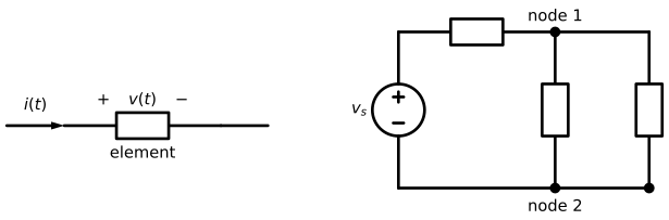
Notice what the right-hand drawing is: a graph, in the discrete-mathematics sense, with elements for edges and nodes for vertices. That observation is not decoration — it is what makes circuit analysis systematic, and it will return in a few pages when Kirchhoff’s laws turn the graph into a solvable system of equations.
Three types of passive element populate these graphs, each with its own symbol (Figure 4.2): the resistor, the capacitor, and the inductor — precisely the three electrical quantities that Lecture 2’s transduction principles ended in.
with schemdraw.Drawing(show=False) as d:
    d += elm.Resistor().right().label('$R$', loc='top').label('resistor', loc='bottom').at((0, 0))
    d += elm.Capacitor().right().label('$C$', loc='top').label('capacitor', loc='bottom').at((5, 0))
    d += elm.Inductor().right().label('$L$', loc='top').label('inductor', loc='bottom').at((10, 0))
d.draw()
Lecture 2’s transduction principles ended in exactly three electrical quantities — a resistance, a capacitance, an inductance — so these three elements are what a sensor is, electrically. Each is defined by its voltage–current relation and by what it does with energy:
\[ v = R\,i, \qquad i = C\,\frac{\mathrm{d}v}{\mathrm{d}t}, \qquad v = L\,\frac{\mathrm{d}i}{\mathrm{d}t}. \tag{4.3}\]
The resistor (\(R\), ohms, \(\Omega\)) opposes the flow of charge: push a current through it and a proportional voltage develops across it. That proportionality is Ohm’s law,
\[ v = i\,R, \tag{4.4}\]
and it says three useful things at once. The relation is linear — double the current, double the voltage — with \(R\) as the slope, so a resistor is fully described by one number. It is instantaneous — the voltage now depends only on the current now, so the resistor has no memory. And it is dissipative: combining Equation 4.4 with \(p = vi\) gives \(p = i^2 R = v^2/R\), always positive — electrical energy leaves the circuit as heat and never comes back. Every resistive sensor from Lecture 2 (strain gauge, RTD, photoresistor) is a resistor whose \(R\) the measurand modulates.
The capacitor (\(C\), farads, F) stores charge on a pair of separated plates, in proportion to the voltage across them:
\[ q = C\,v. \tag{4.5}\]
Differentiating Equation 4.5 (and recalling \(i = \mathrm{d}q/\mathrm{d}t\)) gives the current form, and integrating that gives the voltage form:
\[ i = C\,\frac{\mathrm{d}v}{\mathrm{d}t}, \qquad v(t) = \frac{1}{C}\int_0^{t} i\,\mathrm{d}t' + v(0). \tag{4.6}\]
Read them as behavior: current flows through a capacitor only while its voltage changes, so it blocks steady conditions and resists sudden voltage jumps; and its voltage is the running integral of the current — the capacitor remembers its history, which is exactly what “storage” means. The energy lives in the electric field between the plates: charging to a voltage \(V\) takes work \(w = \int_0^V Cv\,\mathrm{d}v = \tfrac12 CV^2\), which the capacitor can give back later.
Charging a capacitor to voltage \(V\) puts charge \(Q = CV\) on it, and each unit of charge crossing a voltage \(V\) carries energy \(\mathrm{d}w = v\,\mathrm{d}q\). So why is the stored energy \(w = \tfrac12 CV^2\) and not \(Q \times V = CV^2\)?
Because the voltage is not \(V\) during the whole process. The first bit of charge arrives when the capacitor is empty (\(v = 0\)) and costs nothing; the last arrives against the full \(v = V\). Each increment costs \(v\,\mathrm{d}q = Cv\,\mathrm{d}v\), and summing them, \(w = \int_0^V Cv\,\mathrm{d}v = \tfrac12 CV^2\) — the average charge “sees” only half the final voltage. (The same integral with \(Li\,\mathrm{d}i\) gives the inductor’s \(\tfrac12 LI^2\).)
The inductor (\(L\), henries, H) is the capacitor’s magnetic mirror image. A changing current through its coil produces a voltage across it,
\[ v = L\,\frac{\mathrm{d}i}{\mathrm{d}t}, \tag{4.7}\]
so it resists sudden current jumps the way a capacitor resists sudden voltage jumps, and it stores energy \(w = \tfrac12 LI^2\) in the magnetic field around its coil. That is exactly why Lecture 2’s capacitive and inductive sensors work: the measurand reshapes the stored field — a moving plate changes where the electric field lives, a moving core changes the magnetic circuit — and the element’s value changes with it.
Note: how the capacitor and inductor behave in time, through the derivatives in Equation 4.3, is the subject of the AC section.
These three elements are not just what sensors are made of. Combined into networks, they can realize essentially any linear transformation of an input signal into an output signal, and the arrangement and magnitudes determine which one. The governing mathematics is a set of coupled linear ordinary differential equations — exactly as for a mass-spring-damper in structural dynamics or a resistance–capacitance model of heat flow through a wall, which is one reason Lecture 2’s seismic mass and this lecture’s circuits keep obeying the same equations. The rest of this lecture studies a handful of these arrangements, starting with the two-resistor kind and building to an interface circuit called the Wheatstone bridge that you will meet in practice constantly.
A circuit, we said, is a graph: the connection pattern among elements. Since each element’s individual behavior is an ordinary differential equation (or, for the resistor, plain algebra), the graph couples those equations together, and analyzing a circuit boils down to solving the resulting system of coupled ODEs simultaneously. What we need is a systematic way to write the coupling down — and it comes from two equalities that fall out of the lumped-element model, or equivalently out of Maxwell’s equations in the low-frequency limit where the wavelength dwarfs the circuit’s length scale. They are Kirchhoff’s circuit laws, stated more than 150 years ago (Dally et al. 1993):
These two laws are all we need to organize the ODE system; everything else is bookkeeping — and the bookkeeping needs a convention. We mark a current arrow and a voltage polarity on each element; with the passive sign convention (current arrow entering the \(+\) terminal), \(p = vi > 0\) means the element absorbs power, and a negative result simply means the true direction is opposite the arrow. Sign errors, not concepts, are what make circuit analysis go wrong.
Two workhorse results fall straight out of the laws rather than needing to be memorized. Resistors in series carry the same current (KCL), so their voltages add (KVL): \(R_e = R_1 + R_2\). Resistors in parallel share the same voltage, so their currents add: \(1/R_e = 1/R_1 + 1/R_2\). The circuit in Figure 4.3 — a source driving \(R_1\) in series with the parallel pair \(R_2 \parallel R_3\) — puts both results in one place; let the two laws do all the work and watch the equivalents emerge on their own.
with schemdraw.Drawing(show=False) as d:
    d += elm.SourceV().up().label('$V_s$')
    d += elm.Resistor().right().label('$R_1$')
    d += elm.Dot()
    d.push()
    d += elm.Resistor().down().label('$R_2$')
    d += elm.Dot()
    d.pop()
    d += elm.Line().right().length(2.2)
    d += elm.Resistor().down().label('$R_3$', loc='right')
    d += elm.Line().left().length(2.2)
    d += elm.Line().left().tox(0)
    d += elm.Label().at((1.15, 1.5)).label('$i_1$')
    d += elm.Label().at((4.35, 1.5)).label('$i_2$')
d.draw()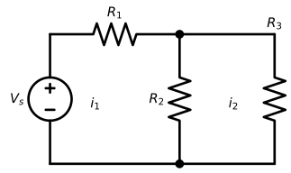
Write KVL around each loop using the loop currents of Figure 4.3 (KCL is built into that bookkeeping: the current through the shared \(R_2\) is \(i_1 - i_2\)):
\[ \text{left loop:}\quad V_s = R_1\,i_1 + R_2\,(i_1 - i_2), \qquad \text{right loop:}\quad 0 = R_2\,(i_2 - i_1) + R_3\,i_2. \]
The right loop gives \(i_2 = \dfrac{R_2}{R_2 + R_3}\,i_1\) — the current-divider rule, incidentally — and substituting it into the left loop collapses everything onto \(i_1\):
\[ V_s = i_1\left(R_1 + R_2 - \frac{R_2^2}{R_2+R_3}\right) = i_1\left(R_1 + \frac{R_2 R_3}{R_2 + R_3}\right). \]
The source sees \(R_1 + R_2 R_3/(R_2+R_3)\) — series resistance plus the parallel combination, obtained rather than memorized. With \(V_s = 12\) V and \(R_1 = 1\ \text{k}\Omega\), \(R_2 = R_3 = 2\ \text{k}\Omega\), the equivalent is \(2\ \text{k}\Omega\), the source supplies 6 mA, and the parallel pair splits it evenly — the numbers of Exercise 1.
A resistor in a circuit is labeled with a current arrow of \(+2\) mA entering its terminal marked \(+\), where the voltage is \(5\) V with respect to the \(-\) terminal. Is it absorbing or delivering power, and how much? What would \(i = -2\) mA have meant?
With current entering the \(+\) terminal, the passive sign convention applies directly: \(p = vi = 5 \times 0.002 = +10\) mW, absorbed (dissipated as heat — it is a resistor, it can do nothing else). Had the analysis returned \(i = -2\) mA, the arrow was simply drawn against the true direction: the element would still absorb \(+10\) mW once the signs are read consistently. A negative absorbed power can only appear on sources — elements that deliver energy.
Lecture 2’s photoresistor and strain gauge both output a resistance, and no analog-to-digital converter reads resistance — something must first turn it into a voltage, and the circuit chosen for that job sets the sensitivity, the linearity, and the noise of everything downstream. Two circuits do almost all of this work in practice, the voltage divider and the Wheatstone bridge, and both fall straight out of the previous section’s laws.
The GL5528 swings from more than 1 MΩ in the dark to 8–20 kΩ at 10 lux, and the simplest way to see that swing on a converter is to put a fixed resistor in series with it across a supply (Figure 4.4). The two resistors carry the same current (KCL), so KVL splits the supply in proportion:
\[ V_{out} = V_s\,\frac{R_2}{R_1 + R_2}. \tag{4.8}\]
with schemdraw.Drawing(show=False) as d:
    d += elm.SourceV().up().label('$V_s$')
    d += elm.Resistor().right().label('$R_1$ (fixed)')
    d += elm.Dot()
    d.push()
    d += elm.Resistor().down().label('$R_2$\n(GL5528)', loc='left')
    d += elm.Line().left()
    d.pop()
    d += elm.Line().right().length(2.4)
    d += elm.Gap().down().label(('+', '$V_{out}$', '−'))
    d += elm.Line().left().length(2.4)
d.draw()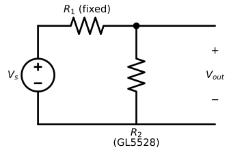
The single design choice hidden in Equation 4.8 — the value of the fixed resistor — determines both how sensitive and how nonlinear the output is in the sensed resistance. Figure 4.5 shows the choice concretely for the GL5528 on a 3.3 V microcontroller supply: a small \(R_1\) concentrates the sensitivity at low (bright) resistances and wastes most of the swing in the dark; a large \(R_1\) does the reverse; and no choice makes the curve straight, because Equation 4.8 is a ratio, not a line. The lesson from Lecture 2 applies verbatim: the circuit, not just the transducer, contributes nonlinearity to the transfer function.
Rldr = np.logspace(3, 6.2, 400)                       # 1 kΩ .. 1.6 MΩ
Vs_ = 3.3
fig, ax = plt.subplots(figsize=(6.2, 3.8))
for Rfix, cc in ((4.7e3, "C0"), (10e3, "C1"), (47e3, "C2")):
    ax.semilogx(Rldr, Vs_ * Rldr / (Rfix + Rldr), color=cc, label=f"$R_1$ = {Rfix/1e3:.1f} kΩ")
    for r10 in (8e3, 20e3):
        ax.plot(r10, Vs_ * r10 / (Rfix + r10), "o", color=cc, ms=4)
ax.axvspan(8e3, 20e3, color="0.85", alpha=0.5)
ax.text(12.5e3, 0.25, "10 lux band", fontsize=8, ha="center")
ax.set_xlabel("GL5528 resistance (Ω)"); ax.set_ylabel("$V_{out}$ (V)")
ax.legend(fontsize=8)
plt.show()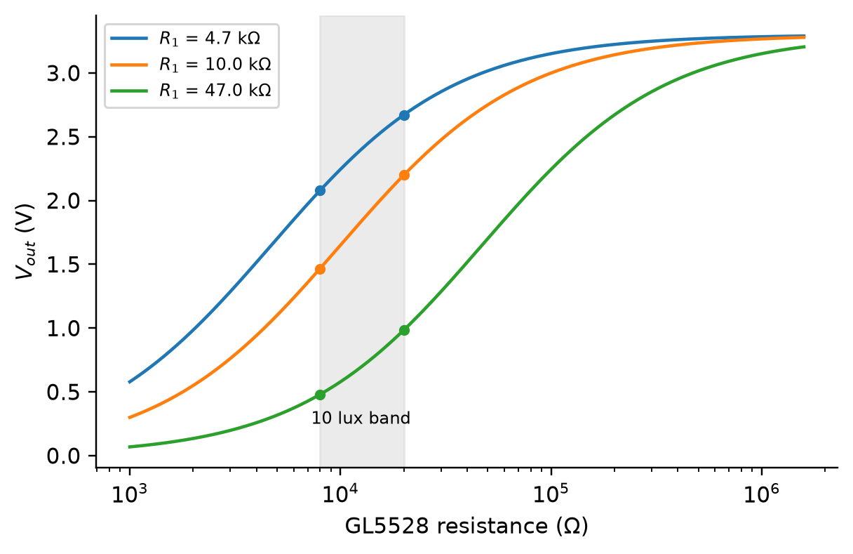
Now put the divider to its real use. Say you have a reliable voltage source \(V\) and a resistive sensor whose resistance \(R_x\) is a function of the phenomenon you care about — a strain gauge on a girder, the GL5528 above, an RTD in a duct. The typical setup for obtaining a useful output voltage is exactly the loop we just studied: place a fixed resistance \(R_1\) in series with \(R_x\) and the source, and measure the voltage drop across \(R_1\) alone (Figure 4.6). Notice that we have moved the probes: with the GL5528 a moment ago we measured across the sensor; here we measure across the fixed resistor. Does it matter? Not fundamentally — the two voltages always add up to \(V\), so either choice carries the full information and one curve is just the other flipped upside down. The choice is practical: probing the fixed resistor lets the output share a reference terminal with the source’s low side (one common “ground,” which the data-acquisition hardware of Lecture 4 will insist on), and it keeps the sensor — often sitting out in the field on long leads — away from the measurement node. KVL gives the divider relation with the sensor upstairs:
\[ V_o \;=\; V\,\frac{R_1}{R_1 + R_x}. \tag{4.9}\]
with schemdraw.Drawing(show=False) as d:
    d += elm.SourceV().up().label('$V$')
    d += elm.Resistor().right().label('$R_x$ (sensor)')
    d += elm.Dot()
    d.push()
    d += elm.Resistor().down().label('$R_1$ (fixed)')
    d += elm.Line().left()
    d.pop()
    d += elm.Line().right().length(2.2)
    d += elm.Gap().down().label(('+', '$V_o$', '−'))
    d += elm.Line().left().length(2.2)
    # impedance-block version
    d += elm.SourceV().up().at((9.5, 0)).label('$V$')
    d += elm.ResistorIEC().right().label('$Z_x$')
    d += elm.Dot()
    d.push()
    d += elm.ResistorIEC().down().label('$Z_1$')
    d += elm.Line().left()
    d.pop()
    d += elm.Line().right().length(2.0)
    d += elm.Gap().down().label(('+', '$V_o$', '−'))
    d += elm.Line().left().length(2.0)
d.draw()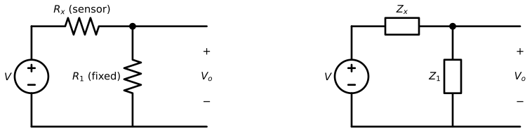
So we have what we wanted: a model \(V_o(R_x)\) relating the voltage we measure to the sensor’s resistance. Two things about it should bother you. First, it is nonlinear — Equation 4.9 is a ratio, and no choice of \(R_1\) straightens it, as Figure 4.5 already showed. Second, and more insidiously, it is biased. Look at the natural operating point where \(R_1\) is chosen close to the sensor’s rest resistance, \(R_1 \approx R_x\): the output sits at \(V_o \approx \tfrac12 V\) before anything has been sensed. For a 120 Ω strain gauge on a 5 V supply, that is a standing 2.5 V on which the signal rides — and the signal itself is tiny: perturbing \(R_x = R(1+\delta)\) around \(R_1 = R\) gives \(V_o \approx \tfrac{V}{2} - \tfrac{V}{4}\delta\). At 1000 µε, a GF 2 gauge has \(\delta = 0.002\), so the information is \(V\delta/4 = 2.5\) mV, riding on 2.5 V of offset. The offset eats the dynamic range of whatever reads \(V_o\) (amplify the signal ×1000 and the offset saturates the amplifier at ×2); and any drift in \(V\) moves the offset by \(\Delta V/2\), indistinguishable from signal.
Can we do better? We would like a circuit whose output is zero when nothing is happening, so that everything downstream — amplifier, converter — works on the signal alone. That wish has a 190-year-old answer.
What if we put two voltage dividers in parallel across the same source, and measure the output between their midpoints (Figure 4.7)? Each midpoint alone carries the offending \(\approx\tfrac12 V\) offset — but their difference subtracts it away, and that is the whole trick.
with schemdraw.Drawing(show=False) as d:
    d += elm.SourceV().up().length(6).label('$V$')
    d += elm.Line().right().length(2)
    d.push()
    d += elm.Resistor().down().label('$R_1$')
    d += (nE := elm.Dot(open=True).label('E', loc='left'))
    d.push()
    d += elm.Resistor().down().label('$R_2$')
    d += elm.Line().left().length(2)
    d.pop()
    d.pop()
    d += elm.Line().right().length(3)
    d += elm.Resistor().down().label('$R_3$')
    d += (nF := elm.Dot(open=True).label('F', loc='right'))
    d.push()
    d += elm.Resistor().down().label('$R_4$')
    d += elm.Line().left().length(3)
    d.pop()
    d += elm.Gap().at(nE.center).to(nF.center).label(('+', '$V_o$', '−'))
d.draw()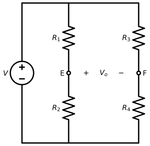
We can place the sensor \(R_x\) in any one of the four resistances — or in two, or in all four — and playing with which arms are fixed and which are sensed gives rise to a whole family of interface circuits. All of them are Wheatstone bridges: ratiometric circuits first developed by Samuel Christie in the 1830s and popularized (and named) a decade later by Charles Wheatstone.
The output takes no new analysis. Each divider’s midpoint voltage is Equation 4.9 with its own labels, and the bridge output is just their difference:
\[ V_o \;=\; V\left(\frac{R_2}{R_1 + R_2} \;-\; \frac{R_4}{R_3 + R_4}\right). \tag{4.10}\]
Does this give a better \(V_o(R_x)\) model? Less biased? Less nonlinear — or even linear? Start with when the output is exactly zero. From Equation 4.10, \(V_o = 0\) whenever the two dividers split the supply identically, which rearranges to the balance condition
\[ R_1 R_4 = R_2 R_3. \tag{4.11}\]
A bridge satisfying it is balanced: zero output, regardless of the supply voltage — balance is a ratio of resistances, so supply drift does not move it. That is our “zero when nothing is happening,” and it is also a measurement method in its own right (adjust a known arm until \(V_o = 0\) and read the unknown from Equation 4.11 — the null method that made this circuit the precision instrument of the nineteenth century (Figliola and Beasley 2019)).
Get a feel for it below: unbalance one arm and watch \(V_o\); enable auto-balance and \(R_4\) follows Equation 4.11; switch to the strain-gauge preset and the strain slider drives \(R_1\) as a 120 Ω, GF 2 gauge would.
Now the deflection question: leave the bridge balanced at rest and let the sensor move one arm. Take three arms fixed at \(R\) and the sensor in the top-left arm, \(R_1 = R_x = R(1+\delta)\) with \(\delta = \Delta R/R\). The sensing divider’s midpoint drops to \(V_E = V\,\dfrac{R}{R(1+\delta) + R} = \dfrac{V}{2+\delta}\) while the fixed divider holds \(V_F = \dfrac{V}{2}\), and their difference is the bridge output:
\[ V_o \;=\; V\left(\frac{1}{2+\delta} - \frac{1}{2}\right) \;=\; -\,V\,\frac{\delta}{4 + 2\delta} \;\approx\; -\,\frac{V}{4}\,\delta. \tag{4.12}\]
Compare this quarter bridge against the lone divider, term by term. The \(\tfrac12 V\) offset is gone — one of the two ratios is exactly \(1/2\) and subtracts it away — so the output starts at zero and the whole measuring chain works on signal. The sensitivity is the same \(V\delta/4\) the divider had (the bridge is not an amplifier). And the response is still nonlinear, through the \(\delta\) in the denominator, and exactly as nonlinear as the divider: the bridge output is the divider’s \(V/(2+\delta)\) minus a constant, and subtracting a constant cannot straighten a curve. Expanding Equation 4.12 for small \(\delta\) shows a relative error of about \(\delta/2\), i.e. 0.1% at 1000 µε for a GF 2 gauge. The sign, incidentally, depends on which arm the sensor occupies: move it from \(R_1\) to \(R_2\) and the output flips.
The numeric headline survives from the divider discussion: a 120 Ω, GF 2 gauge at 1000 µε on 5 V produces \(|V_o| \approx 2.5\) mV — now riding on zero instead of on 2.5 V. That number is why Lecture 5’s instrumentation amplifier exists.
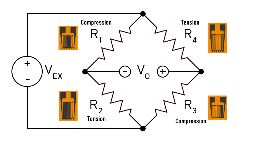
Can the bridge be forced linear? Yes — use the structure, not just one arm. Bond gauges to both faces of a bending member: a cantilever beam with gauges on top (stretched, \(+\delta\)) and bottom (compressed, \(-\delta\)) supplies matched pairs of opposite sign. Wire tension gauges into \(R_2\) and \(R_3\) and compression gauges into \(R_1\) and \(R_4\) — the full bridge — and Equation 4.10 collapses:
\[ V_o = V\left(\frac{1+\delta}{2} - \frac{1-\delta}{2}\right) = V\,\delta \qquad\text{— exactly linear, and four times the quarter-bridge output.} \tag{4.13}\]
As a bonus, a uniform temperature change moves all four gauges by the same \(+\delta_T\), which cancels in both ratios: the full bridge rejects temperature for free — Lecture 2’s “dummy gauge” trick taken to its logical conclusion. This is exactly how commercial load cells are built (Figure 4.8).
eps = np.linspace(0, 5000, 200)                # µε
delta = 2.0 * eps * 1e-6                       # GF = 2
V_n = 5.0
q_exact = V_n * delta / (4 + 2*delta) * 1e3    # mV
fbr = V_n * delta * 1e3
fig, ax = plt.subplots(figsize=(6.2, 3.9))
ax.plot(eps, q_exact, label="quarter (exact)")
ax.plot(eps, fbr, label="full")
ax.set_xlabel("strain (µε)"); ax.set_ylabel("$|V_o|$ (mV)"); ax.legend(fontsize=8, loc="upper left")
axi = ax.inset_axes([0.6, 0.16, 0.36, 0.38])
axi.plot(eps[1:], (q_exact[1:]/(V_n*delta[1:]/4*1e3) - 1) * 100, color="C0")
axi.set_xlabel("µε", fontsize=7); axi.set_ylabel("quarter nonlin. (%)", fontsize=7)
axi.tick_params(labelsize=7)
plt.show()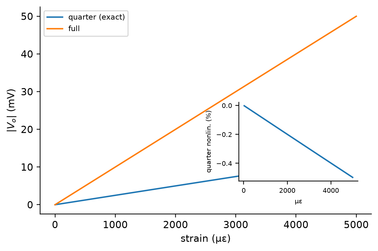
You swap the excitation supply’s polarity, so \(V\) becomes \(-V\). What happens to the bridge output \(V_o\), and what happens to the balance condition?
The output flips sign — Equation 4.10 is proportional to \(V\) — so a bridge reading \(+2.5\) mV now reads \(-2.5\) mV. The balance condition Equation 4.11 does not change at all: it is a ratio of resistances with no \(V\) in it. Output and balance are different kinds of things — a signed difference and a ratio — and only the first knows which way the supply points.
The CR3110 current transformer outputs a 60 Hz sinusoid, a bridge’s vibration is a sum of sinusoids, and the \(\mathrm{d}v/\mathrm{d}t\) in the capacitor’s defining relation means that for such signals the DC toolkit stops working — every element now shifts the signal in time as well as scaling it. Phasors and impedance are the two ideas that make the DC toolkit work again, unchanged, for any sinusoidal signal — and they work because a linear circuit is the same kind of object your structural dynamics course called \(m\ddot{x} + c\dot{x} + kx = f(t)\): a linear time-invariant system, characterized the same way whatever physics it is made of.
The output of a linear time-invariant (LTI) circuit is the convolution of its input with the circuit’s impulse response — the same statement that holds for a linear structure under dynamic load or a wall under a temperature history. Sinusoids are the special inputs that emerge as sinusoids at the same frequency, only scaled and shifted (that is, eigenfunctions of LTI systems) — which is why phasors and impedance work at all: analyzing one frequency at a time diagonalizes the system. Lecture 6 makes this formal.
A sinusoid \(A\cos(\omega t + \phi)\) is fully described by two numbers, its amplitude and its phase, yet carrying the cosine through every derivative of a circuit equation is what makes AC analysis look hard. Euler’s formula, \(e^{j\theta} = \cos\theta + j\sin\theta\), fixes that: write the signal as the real part of
\[ A\,e^{j\phi}\,e^{j\omega t}, \tag{4.14}\]
and the whole time dependence sits in the common factor \(e^{j\omega t}\), whose derivative is just \(j\omega\,e^{j\omega t}\). Differentiation has become multiplication by \(j\omega\), so the differential equations of Equation 4.3 become algebra on the complex amplitude \(A e^{j\phi}\) — the phasor — which you can draw as an arrow of length \(A\) at angle \(\phi\) in the complex plane. Every arrow in a circuit rotates at the same \(\omega\); only lengths and relative angles differ, and those are what we solve for.
That is the entire toolkit this lecture uses.
Once signals are phasors, the natural question is whether a single number per element can play the role \(R\) plays for DC. It can. Substituting Equation 4.14 into each relation of Equation 4.3 and cancelling the common \(e^{j\omega t}\):
\[ Z_R = R, \qquad Z_C = \frac{1}{j\omega C}, \qquad Z_L = j\omega L, \tag{4.15}\]
and Ohm’s law generalizes to \(V = Z\,I\) on phasors. With that, everything from the DC sections carries over verbatim — KVL, KCL, series and parallel combination, the divider, the bridge — with complex arithmetic replacing real. The magnitude of \(Z\) says how much the element impedes; the angle says how much it shifts the signal in time (\(90°\) ahead for the inductor, \(90°\) behind for the capacitor, by rule 4 of the callout).
The frequency dependence is the new ingredient, and it is dramatic. A 1 µF capacitor presents \(|Z_C| = 1/(\omega C)\):
| frequency | 1 Hz | 60 Hz | 10 kHz |
|---|---|---|---|
| \(\lvert Z_C \rvert\), 1 µF | 159 kΩ | 2.65 kΩ | 15.9 Ω |
“A capacitor blocks DC and passes high frequencies” is this table in words — and the inductor runs it in reverse, \(|Z_L| = \omega L\) growing from a short at DC toward an open circuit at high frequency (which is all we will need of inductors beyond the CT).
fig, ax = plt.subplots(figsize=(5.4, 4.0))
ax.axhline(0, color="0.8", lw=0.8); ax.axvline(0, color="0.8", lw=0.8)
ax.annotate("", (1.0, 0), (0, 0), arrowprops=dict(arrowstyle="->", color="C0", lw=2))
ax.text(1.02, 0.05, "$Z_R = R$", color="C0")
for w_, alpha in ((0.35, 1.0), (0.6, 0.55), (1.0, 0.3)):
    ax.annotate("", (0, 1/w_ * 0.55), (0, 0), arrowprops=dict(arrowstyle="->", color="C2", lw=2, alpha=alpha))
    ax.annotate("", (0, -1/w_ * 0.55), (0, 0), arrowprops=dict(arrowstyle="->", color="C1", lw=2, alpha=alpha))
ax.text(0.05, 1.35, "$Z_L = j\\omega L$\n(grows with $\\omega$)", color="C2")
ax.text(0.05, -1.55, "$Z_C = 1/(j\\omega C)$\n(shrinks as $\\omega$ grows)", color="C1")
ax.set_xlim(-0.6, 1.9); ax.set_ylim(-1.85, 1.85)
ax.set_xlabel("real part (Ω)"); ax.set_ylabel("imaginary part (Ω)")
ax.set_xticks([]); ax.set_yticks([])
plt.show()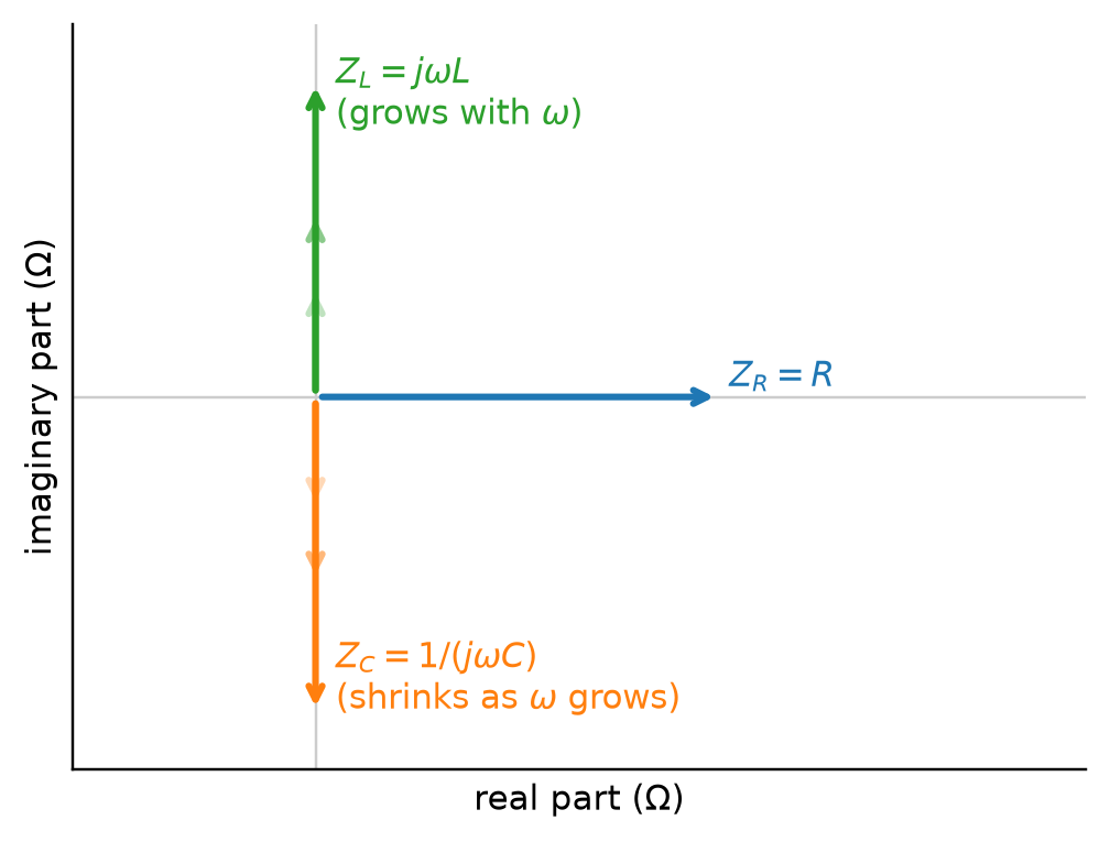
At what frequency do a 10 kΩ resistor and a 1 µF capacitor have equal impedance magnitude? And when they do, what is the phase between their voltages if they carry the same current?
\(|Z_C| = 1/(2\pi f C) = 10\ \text{k}\Omega\) gives \(f = 1/(2\pi \times 10^4 \times 10^{-6}) \approx 15.9\) Hz. Equal magnitude, but not equal behavior: with the same current, the resistor’s voltage is in phase with it while the capacitor’s lags by \(90°\) — the two voltages are \(90°\) apart. Impedances are complex numbers; comparing only their magnitudes discards half the information, as the RLC exercise below shows numerically.
Time to collect the promise made in Section 4.4.2: the divider relation survives when the blocks hold impedances instead of resistances. Put a capacitor in the measured slot (\(Z_1 = 1/(j\omega C)\)) with a resistor upstream (\(Z_x = R\)), and the divider formula on phasors, \(V_o/V_i = Z_1/(Z_x + Z_1)\), gives
\[ \frac{V_o}{V_i} \;=\; \frac{1/(j\omega C)}{R + 1/(j\omega C)} \;=\; \frac{1}{1 + j\omega RC}, \tag{4.16}\]
To read magnitude and phase off Equation 4.16, put it in rectangular form by multiplying numerator and denominator by the conjugate \(1 - j\omega RC\):
\[ \frac{V_o}{V_i} = \frac{1 - j\omega RC}{1 + (\omega RC)^2}, \qquad \left|\frac{V_o}{V_i}\right| = \sqrt{\mathrm{Re}^2 + \mathrm{Im}^2} = \frac{1}{\sqrt{1 + (\omega RC)^2}}, \qquad \angle\frac{V_o}{V_i} = \arctan\frac{\mathrm{Im}}{\mathrm{Re}} = -\arctan(\omega RC). \]
The circuit has quietly become frequency-selective: at \(\omega RC = 0.1\) the output is barely touched (99.5%, \(-5.7°\)); at \(\omega RC = 1\) it is down to 70.7% and lagging \(45°\); at \(\omega RC = 10\) only a tenth survives. A divider with a capacitor in it is a filter — nobody asked it to be one — and the next section gives this two-component circuit the full treatment it has earned.
The two arrows below are the phasors of \(V_i\) (fixed) and \(V_o\) for the RC divider; slide the frequency and watch the output shrink and swing behind.
A 100 Ω resistor, a 100 mH inductor, and a 47 µF capacitor are in series across a 10 V (amplitude), 60 Hz source (Figure 4.11). Find the total impedance, the current phasor, and the voltage across each element — then explain how the element voltage magnitudes can add up to more than 10 V.
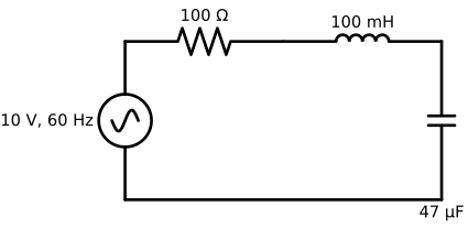
\(Z_L = j\,2\pi(60)(0.1) = j37.7\ \Omega\), \(Z_C = -j/(2\pi \times 60 \times 47\,\mu\text{F}) = -j56.44\ \Omega\), so \(Z = 100 - j18.74\ \Omega\), \(|Z| = 101.7\ \Omega\). Current: \(I = 10/Z = 98.3\) mA at \(+10.6°\). Element voltages: \(|V_R| = 9.83\) V, \(|V_L| = 3.71\) V, \(|V_C| = 5.55\) V — summing to 19.1 V. No contradiction: these are phasor magnitudes, and the phasors point in different directions (\(V_L\) and \(V_C\) nearly opposite). Added as complex numbers they return exactly the 10 V source, as KVL demands. Adding magnitudes of things with phase is the classic AC mistake.
One circuit appears in every later lecture — the anti-aliasing filter of Lecture 5, the ADXL335’s bandwidth-setting capacitor, the first-order sensor of Lecture 2 — and it is worth studying properly once. A resistor and a capacitor in series have a time-domain story (charging) and a frequency-domain story (filtering), and they are the same story told two ways.
Lecture 2 asserted that a first-order sensor obeys \(\tau\,\dot y + y = x\) and quoted its 63% and 95% milestones without proof; an RC circuit is that same equation with a circuit you can build for a dollar. KVL around the loop of Figure 4.12, with the capacitor’s relation \(i = C\,\mathrm{d}v_C/\mathrm{d}t\), gives
\[ RC\,\frac{\mathrm{d}v_C}{\mathrm{d}t} + v_C = v_{in}, \tag{4.17}\]
first-order with time constant \(\tau = RC\). Solve it for a step input — \(v_{in}\) jumps from 0 to \(V\) at \(t = 0\) with the capacitor initially empty — by separating the variables: gather everything involving the unknown \(v_C\) on one side and everything involving \(t\) on the other. Rearranging Equation 4.17,
\[ \tau\,\frac{\mathrm{d}v_C}{\mathrm{d}t} = V - v_C \qquad\Longrightarrow\qquad \frac{\mathrm{d}v_C}{V - v_C} = \frac{\mathrm{d}t}{\tau}, \]
a move that is legal because \(V - v_C\) is never zero on the way up. Now integrate both sides from the start (\(t = 0\), \(v_C = 0\)) to an arbitrary later moment — a dummy variable \(u\) keeps the limits honest — and evaluate the left side, which is \(-\ln(V - u)\):
\[ \int_0^{v_C}\frac{\mathrm{d}u}{V - u} = \int_0^{t}\frac{\mathrm{d}t'}{\tau} \qquad\Longrightarrow\qquad \ln\frac{V}{V - v_C} = \frac{t}{\tau}. \]
Exponentiating both sides and solving for \(v_C\):
\[ v_C(t) = V\left(1 - e^{-t/\tau}\right), \tag{4.18}\]
and there are Lecture 2’s milestones, no longer quoted but derived: \(1 - e^{-1} = 63.2\%\) at \(t = \tau\), \(95.0\%\) at \(3\tau\). Discharging from \(V\) is the mirror case, \(v_C = V e^{-t/\tau}\). Physically the story is the loop fighting the field: the resistor limits how fast charge can arrive, the capacitor’s growing voltage reduces what pushes the charge, and the approach to the final value is exponential because the push is proportional to the remaining gap.
with schemdraw.Drawing(show=False) as d:
    d += elm.SourceV().up().label('$v_{in}$')
    d += elm.Resistor().right().label('$R$')
    d += elm.Dot()
    d.push()
    d += elm.Capacitor().down().label('$C$', loc='left')
    d += elm.Line().left()
    d.pop()
    d += elm.Line().right().length(2.4)
    d += elm.Gap().down().label(('+', '$v_C$ (low-pass)', '−'))
    d += elm.Line().left().length(2.4)
d.draw()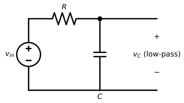
from scipy.integrate import solve_ivp
t = np.linspace(0, 60e-3, 1201)
fig, ax = plt.subplots(figsize=(6.2, 3.6))
for tau_, cc in ((1e-3, "C0"), (10e-3, "C1"), (100e-3, "C2")):
    num = solve_ivp(lambda tt, y: (1.0 - y)/tau_, [0, 60e-3], [0.0], t_eval=t, rtol=1e-8).y[0]
    ax.plot(t*1e3, num, color=cc, label=f"τ = {tau_*1e3:g} ms")
    ax.plot(t[::80]*1e3, 1 - np.exp(-t[::80]/tau_), ".", color=cc, ms=3)   # analytic overlay
ax.plot([10, 30], [1-np.exp(-1), 1-np.exp(-3)], "ks", ms=4)
ax.annotate("63.2% at τ", (10, 0.632), xytext=(16, 0.45), fontsize=8, arrowprops=dict(arrowstyle="->"))
ax.annotate("95.0% at 3τ", (30, 0.950), xytext=(36, 0.78), fontsize=8, arrowprops=dict(arrowstyle="->"))
ax.set_xlabel("time (ms)"); ax.set_ylabel("$v_C / V$"); ax.legend(fontsize=8, loc="lower right")
plt.show()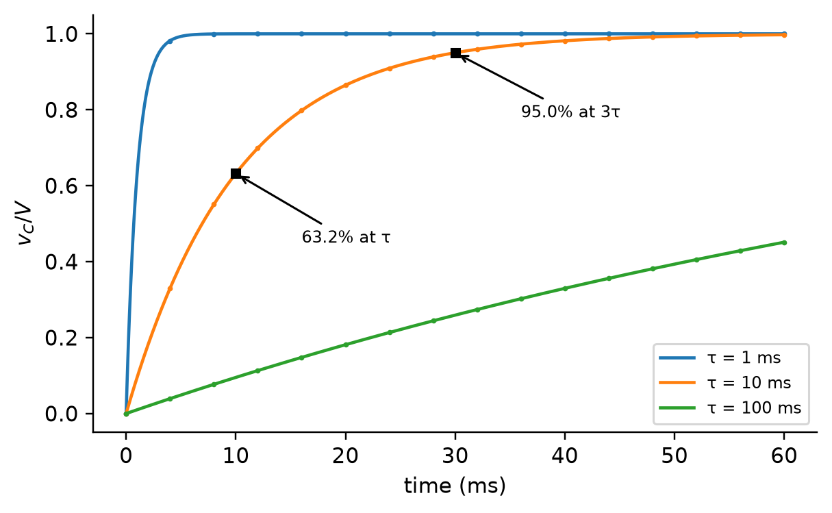
The AC divider already found \(V_o/V_i = 1/(1 + j\omega RC)\) for exactly this circuit, so we hold two descriptions of one object and should understand how they relate. The magnitude \(1/\sqrt{1 + (\omega RC)^2}\) equals \(1/\sqrt{2}\) — the output power halved — at the cutoff frequency
\[ f_c = \frac{1}{2\pi RC} = \frac{1}{2\pi \tau} \approx \frac{0.159}{\tau}, \tag{4.19}\]
which is Fraden’s \(0.159/\tau\) from Lecture 2 with its origin now visible, and the ADXL335’s datasheet formula \(f = 1/(2\pi \cdot 32\ \text{k}\Omega \cdot C)\) verbatim — the accelerometer’s 32 kΩ output resistance and your added capacitor simply form this circuit. A fast time constant is a high cutoff and vice versa: the two descriptions carry the same single parameter \(\tau = RC\).
The landmarks of Table 4.3 are the whole vocabulary of the decibel; the callout below explains where they come from and lets you hear them.
| amplitude ratio | decibels | power ratio |
|---|---|---|
| \(\times\sqrt{2}\) | \(+3\) | \(\times 2\) |
| \(\times 2\) | \(+6\) | \(\times 4\) |
| \(\times 10\) | \(+20\) | \(\times 100\) |
| \(\times 100\) | \(+40\) | \(\times 10^4\) |
| \(\times 1000\) | \(+60\) | \(\times 10^6\) |
| \(\div\sqrt{2}\) | \(-3\) | \(\div 2\) |
| \(\div 2\) | \(-6\) | \(\div 4\) |
| \(\div 10\) | \(-20\) | \(\div 100\) |
The quantities in a measurement chain span a factor of a million or more: microvolts of noise at one end, volts of supply at the other, and a 24-bit converter with sixteen million levels in between. What matters at every stage is not a level but a ratio: the gain of an amplifier, the attenuation of a filter, the signal against its noise. Multiplying such ratios down a chain of stages is hopeless to do in your head; the decibel is a ruler on which multiplying becomes adding, and the rest of this book speaks it fluently.
For an amplitude ratio (voltages, currents, accelerations) and for a power ratio,
\[ \text{dB} = 20\log_{10}\frac{V_o}{V_i} = 10\log_{10}\frac{P_o}{P_i}, \tag{4.20}\]
two definitions that agree because power goes as the square of amplitude, and \(\log_{10}\) of a square is twice the log. Zero decibels is “unchanged”; negative decibels is attenuation. Six landmarks carry almost every use you will meet (Table 4.3), and the one at \(-3\) dB is the cutoff of Equation 4.19: an amplitude ratio of \(1/\sqrt{2}\), which is half the power, which is why datasheets quote bandwidth “at \(-3\) dB”.
Because logarithms turn products into sums, stages in a chain add in decibels. An amplifier with a gain of 100 (40 dB) followed by a filter operating at its cutoff (\(-3\) dB) has a combined gain of 37 dB, which is a factor of \(10^{37/20} \approx 71\): the same answer as \(100 \times 0.707\), arrived at without a multiplication.
Slide the level and watch the same ratio on a linear axis, where anything below \(-40\) dB vanishes, and on a logarithmic axis, where every 20 dB is one tick. The button plays a reference tone and then the same tone at the chosen level: the ear, like the ruler, hears ratios, and \(-6\) dB is only slightly softer while \(-30\) dB is faint.
Now a chain. Set the gain of each stage and read the two totals side by side: the ratios multiply, the decibels add.
You will meet each landmark again soon: the \(-3\) dB of the cutoff in this section, the 6 dB that one converter bit buys in Lecture 4, the 20 dB per decade of a Bode plot’s slope in Lecture 5, and the 13 and 31 dB that separate a window’s side lobes from its peak in Lecture 6.
A filter’s datasheet says the response is \(-3\) dB at the cutoff and \(-40\) dB at ten times the cutoff. A 1 V sinusoid enters at each of those frequencies. What amplitude leaves?
\(10^{-3/20} = 0.71\) V at the cutoff, and \(10^{-40/20} = 0.01\) V a decade above it: the second number is why the \(-40\) dB figure, not the cutoff, is what an anti-aliasing design in Lecture 5 will care about.
One circuit, two views: slide \(R\) and \(C\) and watch the step response and the frequency response move together — a slower charge is a lower cutoff, always.
Swap the positions of R and C and the same two components pass high frequencies instead — the circuit’s function is a matter of where you take the output. Taking \(v_C\) gives the low-pass filter just studied: it smooths and delays, which is what an anti-aliasing filter wants (Lecture 5) and what your thermometer’s sheath does whether you want it or not. Taking \(v_R = v_{in} - v_C\) gives a high-pass filter, \(|V_o/V_i| = \omega RC/\sqrt{1+(\omega RC)^2}\): it blocks DC entirely and passes fast changes — which is why a piezoelectric sensor, read through a charge amplifier, has a lower cutoff frequency as well as an upper one, closing the loop opened in Lecture 2 (the details live in the linked article; the shape of the behavior is just this curve).
fr = np.logspace(-2, 2, 400)                   # f / f_c
lp = 1/np.sqrt(1 + fr**2)
hp = fr/np.sqrt(1 + fr**2)
fig, ax = plt.subplots(figsize=(6.2, 3.6))
ax.loglog(fr, lp, label="low-pass ($v_C$)")
ax.loglog(fr, hp, label="high-pass ($v_R$)")
ax.axvline(1, color="0.7", ls=":"); ax.axhline(1/np.sqrt(2), color="0.7", ls=":")
ax.annotate("$f_c$: both at $1/\\sqrt{2}$ (−3 dB)", (1, 1/np.sqrt(2)), xytext=(2.4, 0.9), fontsize=8,
            arrowprops=dict(arrowstyle="->"))
ax.set_xlabel("$f / f_c$"); ax.set_ylabel("$|V_o / V_i|$"); ax.set_ylim(5e-3, 1.6); ax.legend(fontsize=8, loc="lower left")
plt.show()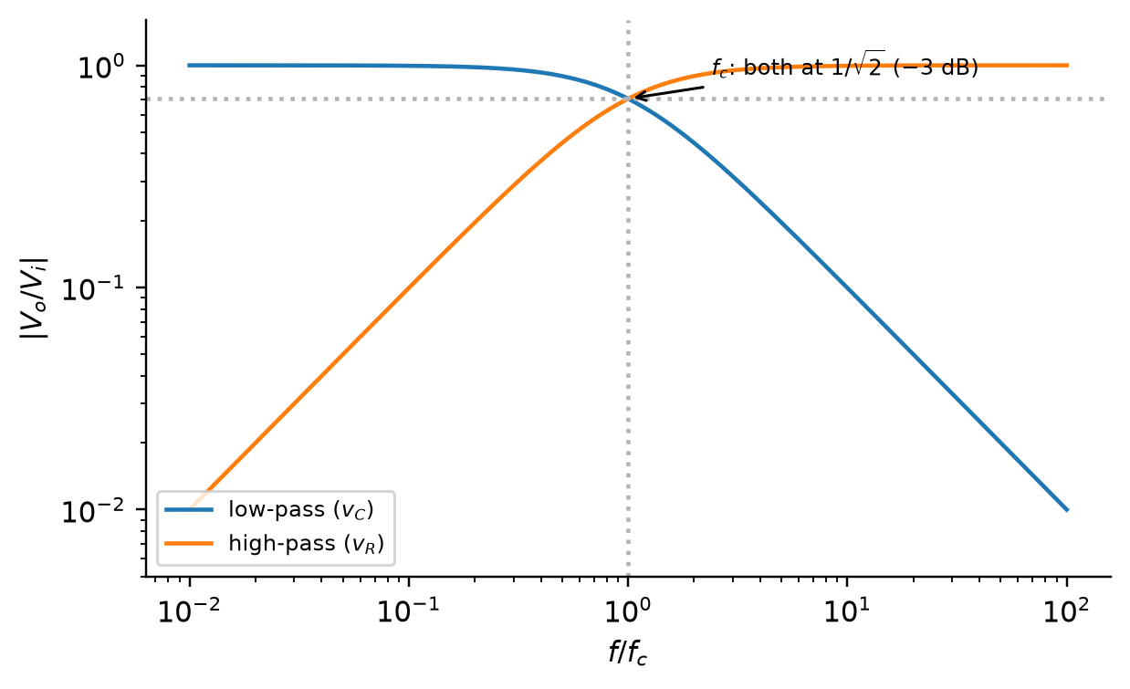
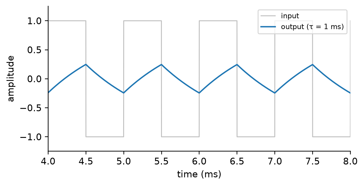
A 1 kHz square wave (period 1 ms) drives an RC low-pass with \(\tau = 1\) ms. Sketch the output.
Each half-period lasts \(0.5\) ms \(= \tau/2\), so the capacitor never gets close to either level: it charges along the first part of an exponential, reverses, and discharges likewise. The output is a small, rounded, nearly triangular wave centered on the square wave’s mean, with a steady-state peak-to-peak swing of \(\tanh(T/4\tau) \approx 24.5\%\) of the input’s — Figure 4.15 shows the worked solution. The mean survives untouched — it is DC, and this is a low-pass. If you connected the ADXL335 with a 10 µF bandwidth capacitor (\(f_c = 0.5\) Hz) to a shaker vibrating at 50 Hz, this is exactly what you did to your data.
Four sections of analysis are only useful if they tell you how to build a measurement chain, and the first thing you do when building one is connect a sensor circuit to an instrument — the moment Lecture 2 warned about under the name “loading.” Thévenin’s theorem reduces any sensor circuit to two numbers, and those two numbers, against the instrument’s input impedance, tell you exactly how much the connection changes the reading.
The bridge of Section 4.4.3 has four resistors and a supply inside it, yet when you wire it to an amplifier you want to treat it as a single thing with two terminals. Thévenin’s theorem says you can: as seen from its terminals, any linear network is equivalent to one ideal voltage source \(V_{Th}\) — the open-circuit voltage at those terminals — in series with one resistance \(R_{Th}\) — the resistance seen looking back in with all sources zeroed (voltage sources shorted, current sources opened). The proof is superposition: a linear network’s terminal behavior is a linear relation \(v = V_{Th} - R_{Th}\,i\), and two measurements (open-circuit voltage, short-circuit current) pin down the line. The dual form — a current source \(V_{Th}/R_{Th}\) in parallel with \(R_{Th}\) — is the Norton equivalent, the natural description of the current transformer.
For the Wheatstone bridge, \(V_{Th}\) is exactly Equation 4.10 (the output we computed was open-circuit — nothing was connected between E and F), and zeroing the supply merges the top and bottom rails, leaving the two dividers as parallel pairs in series:
\[ R_{Th} = \frac{R_1 R_2}{R_1 + R_2} + \frac{R_3 R_4}{R_3 + R_4}, \tag{4.21}\]
which for equal 350 Ω arms is just 350 Ω (Figliola and Beasley 2019). If you distrust shortcuts, do it the long way: connect a load \(R_L\) between E and F and write KCL at each midpoint,
\[ \frac{V - V_E}{R_1} - \frac{V_E}{R_2} + \frac{V_F - V_E}{R_L} = 0, \qquad \frac{V - V_F}{R_3} - \frac{V_F}{R_4} + \frac{V_E - V_F}{R_L} = 0. \]
Solving the pair for \(V_E - V_F\) and rearranging, the loaded output takes exactly the divider form \(V_{load} = V_{Th}\,\dfrac{R_L}{R_L + R_{Th}}\), with \(V_{Th}\) given by Equation 4.10 and \(R_{Th}\) by Equation 4.21 — the two-number summary was hiding in the algebra all along.
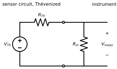
Connect a voltmeter with 10 kΩ input resistance to the midpoint of a 10 kΩ/10 kΩ divider and it reads a third low; connect a 10 MΩ meter and it is right to 0.05% — same circuit, same “true” voltage, different answer. There is no mystery once the source is in Thévenin form (Figure 4.16): the instrument’s input resistance \(R_{in}\) forms another divider with \(R_{Th}\), so
\[ V_{meas} = V_{Th}\,\frac{R_{in}}{R_{Th} + R_{in}}, \qquad \text{relative error} = \frac{R_{Th}}{R_{Th} + R_{in}}, \tag{4.22}\]
the loading error of Lecture 2, now with a formula (Figliola and Beasley 2019). The rule of thumb follows immediately: \(R_{in} = 10\,R_{Th}\) leaves a 9% error, \(100\,R_{Th}\) leaves 1%, and a good voltage-measuring instrument simply makes \(R_{in}\) enormous. Figure 4.17 places our running examples on that curve — and note the CR3110’s burden resistor is the deliberate exception: a current-output sensor wants its load, chosen by design rather than suffered.
ratio = np.logspace(0, 5, 300)
err = 1/(1 + ratio) * 100
fig, ax = plt.subplots(figsize=(6.2, 3.6))
ax.loglog(ratio, err)
for rr, name in ((1e6/350, "bridge → in-amp"), (1e5/5e3, "GL5528 → MCU ADC"), (1e7/5e3, "GL5528 → bench meter")):
    ax.plot(rr, 1/(1+rr)*100, "o", ms=5)
    below = name.startswith("bridge")                      # the bridge and bench-meter markers sit close together
    ax.annotate(name, (rr, 1/(1+rr)*100), xytext=(rr*(0.6 if below else 1.3), 1/(1+rr)*100*(0.25 if below else 3.2)), fontsize=8, ha="center")
ax.set_xlabel("$R_{in} / R_{Th}$"); ax.set_ylabel("loading error (%)")
plt.show()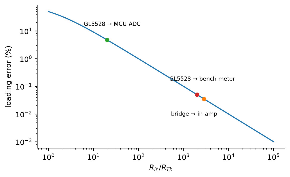
The same rule holds with impedance in place of resistance, and it explains a datasheet line skipped in Lecture 2: the ADXL335’s 32 kΩ output resistance is its \(R_{Th}\), and the bandwidth capacitor you attach forms the RC filter of Equation 4.19 with it — the datasheet formula is nothing but this section applied by the manufacturer on your behalf. The general design rule for a measurement chain: voltage signals want high input impedance downstream (take nearly all the voltage, draw nearly no current), and current signals want low — the CT’s burden resistor and a photodiode’s transimpedance stage are both deliberately small loads for current-output devices.
If you have met impedance matching in an antennas, RF, or audio context, forget it for a moment: the condition \(R_{in} = R_{Th}\) maximizes power transfer, and it does so while throwing away half the voltage and loading the source heavily. A measurement chain almost never wants power from the sensor — it wants the voltage (or the current) reported faithfully, which calls for \(R_{in} \gg R_{Th}\) (or \(\ll\), for current). Apply the RF rule to a strain-gauge bridge and you halve your 2.5 mV signal and double your error budget for nothing.
A Wheatstone bridge with four 350 Ω arms feeds an instrumentation amplifier with 1 MΩ input resistance. Is loading a concern? What if the amplifier’s input resistance were 10 kΩ?
First find the source resistance. By Equation 4.21 each divider contributes its two arms in parallel, \(\dfrac{350 \times 350}{350 + 350} = 175\ \Omega\) per side, and the two sides add in series: \(R_{Th} = 175 + 175 = 350\ \Omega\) — not \(4 \times 350\). Into 1 MΩ: error \(= 350/(350 + 10^6) \approx 0.035\%\), negligible against the bridge’s other errors. Into 10 kΩ: \(\approx 3.4\%\) — a 1000 µε reading reported as ≈ 966 µε, a systematic error larger than everything in Lecture 2’s datasheet section combined. The habit to build: compute \(R_{Th}\) before judging the instrument.
Open the ADXL335 and CR3110-3000 datasheets and find every line that is a source or input impedance in disguise — output resistance, secondary DC resistance, burden resistor guidance, maximum output voltage. For each, say which rule from this section it is enforcing, and whether the quantity wants to be large or small.
Maxwell’s equations, in the \(D \ll \lambda\) limit, hand us the lumped-element model; two conservation laws and three element relations then analyze any circuit. A divider turns a resistance into a voltage but leaves the signal riding on a \(\tfrac12 V\) offset; the Wheatstone bridge — two dividers minus each other — removes the offset, and with enough active arms removes the nonlinearity and the temperature sensitivity too. Phasors and impedance make the same tools work for signals that move; the RC pair is a clock in the time domain and a filter in the frequency domain — the same object either way; and Thévenin’s theorem collapses any of it to two numbers that decide whether connecting the next stage will corrupt the reading. Lecture 4 sends the output of that next stage into a digital converter, and Lecture 5 builds the amplifier that the bridge’s 2.5 mV has been asking for since the middle of this page.
\(R_2 \parallel R_3 = 1\) kΩ, so \(R_e = 2\) kΩ and the source current is \(i_1 = 12/2000 = 6\) mA. The node between them sits at \(12 - 6\,\text{mA} \times 1\,\text{k}\Omega = 6\) V, so \(i_2 = i_3 = 3\) mA (symmetry, and KCL checks: \(3+3=6\)). Powers: \(P_1 = i_1^2 R_1 = 36\) mW; \(P_2 = P_3 = i_2^2 R_2 = 18\) mW. Total 72 mW \(= 12\,\text{V} \times 6\,\text{mA}\), as energy conservation demands.
Root bending stress: \(\sigma = 6FL/(bh^2) = 6 \times 10 \times 0.3 / (0.025 \times 0.006^2) = 20\) MPa, so \(\varepsilon = \sigma/E = 100\) µε, equal and opposite on the two faces. With \(R_1 = R(1-\delta)\) and \(R_2 = R(1+\delta)\), the left midpoint sits at \(V(1+\delta)/2\) and the right at \(V/2\), so \(V_o = \tfrac{V}{2}\,\delta = \tfrac{V}{2}\,\text{GF}\,\varepsilon = 2.5 \times 2.1 \times 100\times10^{-6} = \mathbf{525\ \mu V}\) — exactly linear, like the full bridge, at half its output (\(V\delta = 1.05\) mV would need gauges on both dividers). Wire the two gauges into \(R_1\) and \(R_3\) instead (same sign of strain in corresponding positions of both dividers) and their contributions cancel: adjacent arms want opposite strains, opposite dividers want like strains. Getting this wiring wrong silently zeroes a working installation.
The series RLC exercise of the AC section (worked there).
Using the ADXL335’s bandwidth formula \(f = 1/(2\pi \cdot 32\ \text{k}\Omega \cdot C)\), choose the capacitor for a 50 Hz cutoff, state the resulting time constant, and describe what a 2 Hz footbridge sway and a 500 Hz truck impact each look like at the output.
\(C = 1/(2\pi \times 32\,\text{k}\Omega \times 50) \approx 99.5\) nF — you would fit the standard 0.1 µF, giving \(f_c = 49.7\) Hz and \(\tau = RC \approx 3.2\) ms. The 2 Hz sway is at \(f/f_c = 0.04\): passed essentially untouched (magnitude 0.999). The 500 Hz impact is at \(f/f_c = 10\): attenuated to about 10% of its amplitude and lagging nearly 90° — present in the data, but small and shifted, exactly the kind of artifact Lecture 2’s “physics shapes your data” section warned about.
\(\delta = 0.002\), so \(|V_{Th}| = 5 \times 0.002/(4+0.004) \approx 2.4975\) mV (Equation 4.12) and \(R_{Th} \approx 350\) Ω (the gauge’s \(350 \times 0.002 = 0.70\) Ω change moves \(R_{Th}\) by only 0.17 Ω). Through 1 MΩ: \(V_{meas} = V_{Th} \times 10^6/(10^6+350) = 2.4966\) mV — an inferred strain low by 0.035%, or 0.35 µε, fine. Through 10 kΩ: \(V_{meas} = 2.4975 \times 10^4/10350 = 2.413\) mV — inferred strain ≈ 966 µε, a 3.4% systematic under-read that no amount of averaging will fix. Loading errors are calibration errors you chose not to prevent.
