10 Lecture 09: Relational Databases and the Entity-Relationship Model
10.1 Lecture Overview
10.1.1 Before You Begin
This lecture opens the database block of the DATA third. Lecture 8 treated one sensor’s record at a time; this one asks how to organize the records of many sensors, the assets they monitor, and the people who look after them. No software is needed: SQL arrives in Lecture 10, and everything here is done with diagrams, small tables, and the notation of sets. The running example is a hypothetical city’s bridge-monitoring program, small enough that every table fits on the page.
10.2 From Time Series to Data Structures
Suppose a city has put accelerometers, strain gauges, and thermometers on its bridges, and every one of them produces a clean time series of the kind Lecture 8 taught you to build. Now the bridge engineer asks: which strain gauges on bridges built before 1950 have gone silent this month, and who inspected those bridges last? No single time series can answer that. The answer lives in how things relate: which sensor is on which bridge, when each bridge was built, which readings belong to which sensor, and which engineer inspected what.
Those relationships are data too, and they are the part that most monitoring programs keep worst: in a spreadsheet tab someone updates by hand, in file names, or in one person’s memory. When the person leaves, or a sensor is moved from one bridge to another and the spreadsheet is not updated, every analysis downstream quietly attaches readings to the wrong structure. That is a sensing failure as real as a broken wire, and it is the reason this course spends five lectures on databases.
This lecture builds three tools, each answering a different need:
- an entity-relationship diagram to design what the database must hold, before any data exists;
- set theory to give a precise meaning to questions like “all sensors except the faulty ones”;
- the relational model and its relational algebra to store the data as tables and query it, with rules that translate the diagram into tables.
10.3 Entity-Relationship Diagrams
Before anyone creates a table, someone has to decide what the database must hold and how its pieces connect. A mistake made there (say, assuming each sensor stays on one bridge forever) is cheap to fix on paper and expensive to fix once three years of readings depend on it. The entity-relationship (E/R) model, introduced by Chen (Chen 1976), is the standard notation for making that decision in the open: a diagram of the things in a system, their properties, and their connections, which engineers, domain experts, and database designers can read and argue over before a single row is stored (Garcia-Molina et al. 2009, Ch. 4).
An E/R diagram describes the structure of the data, not the data itself. No database system stores E/R diagrams directly; the diagram is converted into tables (Section 10.7), and it earns its keep by making the design decisions visible while they are still cheap to change.
10.3.1 A First Example: Monitoring a Bridge Network
Vocabulary is easier to learn when it names parts of something familiar, so we start from a picture and name its parts afterwards. Figure 10.1 records two kinds of things, bridges and sensors, and one fact that connects them: a sensor monitors a bridge.
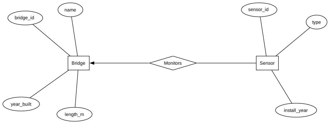
The diagram uses three shapes, following Garcia-Molina, Ullman, and Widom:
- rectangles are entity sets (Bridge, Sensor);
- ovals are attributes (
name,year_built,type, …); - diamonds are relationships (Monitors), with edges to the entity sets they connect.
The arrow from Monitors into Bridge carries a constraint, and underlined attributes are keys. The next two subsections make those precise.
10.3.2 Entity Sets and Attributes
To store facts about “the Harbor Bridge” or “strain gauge S3”, we first need to say what kind of thing each is and what we want to know about it. An entity is one such thing, abstract or physical: a bridge, a sensor, an engineer, an inspection. An entity set is a collection of entities of the same kind; Bridge is the set of all bridges the city monitors, and each bridge is one entity in it. An entity set resembles a class in object-oriented programming, with the difference that it describes only data, not operations.
Attributes are the properties every entity of the set has: each bridge has a name, a year_built, and a length_m. In the E/R model used in this course, attribute values are atomic: a string, an integer, a real number, a date, never a list or a set (Garcia-Molina et al. 2009, Ch. 4). That restriction is deliberate, because it is the one the relational model imposes too.
A key is a set of attributes whose values no two entities of the set can share; it is how the database tells one entity from another. Keys are underlined in the diagram. name looks like a candidate for Bridge, until two agencies both have a “Riverside Bridge”; a bridge_id issued by the city, like an employee ID or a vehicle registration number, exists precisely to be a key. Every entity set must have one.
NoteOther notations: multi-valued and derived attributes
You will meet E/R diagrams, especially in the notation of Elmasri and Navathe, with double ovals for multi-valued attributes (a bridge built of several materials) and dashed ovals for derived ones (a bridge’s age, computable from year_built). The atomic-attribute model handles both without new symbols: a multi-valued property becomes its own entity set connected by a relationship (Bridge — Built_Of — Material), and a derived value is simply not stored, because storing it invites the copy and the source to disagree.
You will also meet crow’s-foot notation in most database tools, with relationships drawn as lines whose ends show “one” or “many” symbols. The concepts are identical; only the drawing differs.
10.3.3 Relationships and Their Multiplicity
Knowing that bridges and sensors exist is useless until we know which sensor is on which bridge, and whether a sensor can be on two bridges at once. A relationship connects two (or more) entity sets. Formally, the current relationship set of Monitors is a set of pairs \((s, b)\), one for each sensor \(s\) that monitors bridge \(b\): a table with one column per participating entity set. Hold on to that “set of pairs”; it is the bridge to Section 10.4.
Most of the design information in a relationship is in its multiplicity. For a binary relationship \(R\) between entity sets \(E\) and \(F\):
- \(R\) is many-one from \(E\) to \(F\) if each member of \(E\) is connected to at most one member of \(F\). It is drawn with an arrow entering \(F\).
- \(R\) is one-one if it is many-one in both directions, drawn with arrows at both ends.
- \(R\) is many-many if it is neither, drawn with no arrows.
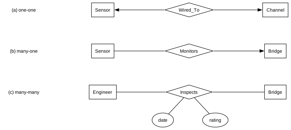
The arrow means at most one, not exactly one. In Figure 10.2 (a), a spare sensor on the shelf is wired to no channel at all, and the diagram allows that. When the design needs “exactly one” (every sensor in the database must be on a bridge that is also in the database) that is a referential integrity constraint, which we will enforce with foreign keys in Section 10.7.
Multiplicity is a statement about the world, not about today’s data. Whether Monitors should be many-one depends on the monitoring program’s policy: if sensors are sometimes moved between bridges and the database must remember where each sensor was, then Monitors is many-many, or better, a history of installations with dates. Getting this wrong is the most common E/R mistake, and it is exactly the kind of mistake the diagram exists to expose.
Relationships can have attributes. In Figure 10.2 (c), the date and rating of an inspection belong neither to the engineer (who inspects many bridges) nor to the bridge (which many engineers inspect); they belong to the pairing of the two.
CautionConcept Check: Two inspections
With the design of Figure 10.2 (c), can the database record that engineer E2 inspected the Harbor Bridge in 2024 and again in 2025?
TipAnswer
No. The relationship set of Inspects is a set of (engineer, bridge) pairs, so the pair (E2, Harbor Bridge) appears at most once, with one date and one rating. Recording a second inspection would overwrite the first. If the history matters (it does, for a bridge), inspections must become entities in their own right: an entity set Inspection with its own date and rating, connected by many-one relationships to Engineer and to Bridge. Relationship attributes fit facts about a pairing that has one value per pair, such as the date an engineer was first assigned to a bridge.
10.3.4 Weak Entity Sets
Reading number 5 means nothing until we know which sensor produced it, because every sensor numbers its readings from 1. The sequence number seq_no is unique only among the readings of one sensor; to identify a reading we need the sensor’s key as well. Readings are a weak entity set: an entity set whose key is made, in part or in whole, of key attributes of another entity set, reached through a many-one relationship (Garcia-Molina et al. 2009, Ch. 4).
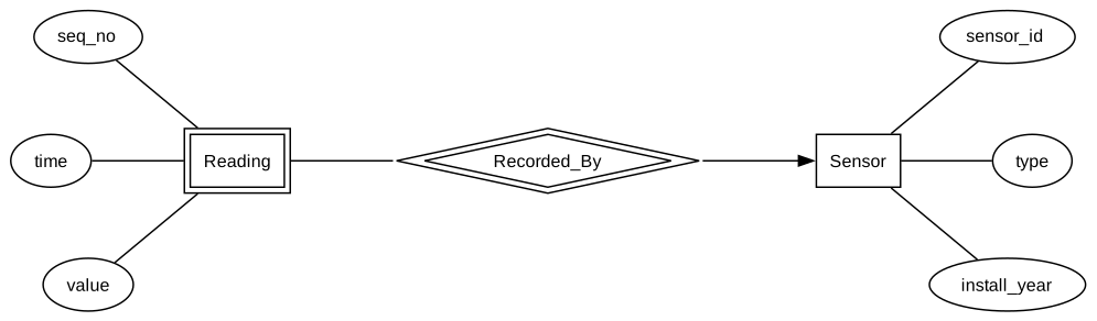
seq_no together with the sensor_id of the sensor that recorded it.
The notation, in Figure 10.3:
- the weak entity set is a double rectangle;
- the relationship that supplies part of its key, the supporting relationship, is a double diamond, and must be many-one from the weak set, with every reading recorded by a sensor that exists in the database;
- the weak set’s own contribution to the key (
seq_no) is underlined, and the rest of the key is the key of the entity set at the arrow’s end.
Weak entity sets arise wherever things are numbered or named within something else: levels within a parking garage, spans within a bridge, timing plans within a traffic-signal controller, readings within a sensor. They also arise when a relationship is promoted to an entity set, as in the concept check above: an inspection is identified by the engineer, the bridge, and the date together.
10.3.5 Roles in Relationships
A road segment connects two intersections, so the same entity set appears twice in one relationship, and “which end is which” becomes ambiguous. When an entity set plays more than one part in a relationship, each edge from the relationship to that entity set is labeled with a role. In Figure 10.4, a traffic model’s road network stores each segment as a relationship between a from intersection and a to intersection, which is how one-way streets and direction-specific travel times are represented.

Roles are needed whenever an entity set is related to itself: the upstream and downstream junctions of a water main, the original and the replacement of a sensor, an engineer and that engineer’s supervisor.
10.3.6 Subclasses and ISA Hierarchies
Suspension, truss, and arch bridges share everything a bridge has, but each has properties the others lack: the diameter of a suspension bridge’s main cables, the configuration of a truss, the rise of an arch. Giving every bridge all three attributes would leave most of them empty, and would let someone record a cable diameter for a truss bridge. A subclass is a special-case entity set whose entities have everything the parent has plus attributes or relationships of their own. It is connected to its superclass by an isa relationship (“a Truss is a Bridge”), drawn as a triangle: one side attached to the subclass, the opposite point connected to the superclass (Garcia-Molina et al. 2009, Ch. 4).
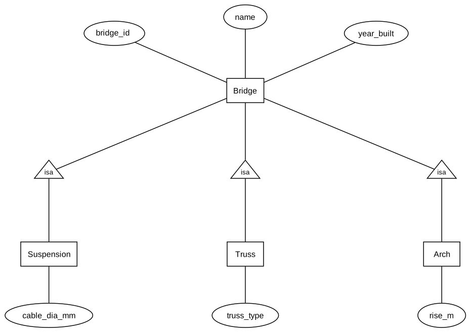
bridge_id, name, and year_built and adds one attribute of its own.
Every isa relationship is one-one: each truss-bridge entity corresponds to exactly one bridge entity. The key of every entity in the hierarchy comes from the root: a truss bridge is identified by its bridge_id, like any other bridge. In the E/R model an entity may have components in several subclasses at once (a bridge that is both a truss and, say, a historic landmark); whether that is allowed is a design decision the diagram should record.
10.3.7 Building an ER Diagram for a Sensing Deployment
Each construct is simple on its own; the skill is recognizing which one a sentence in a requirements description calls for. Here are the requirements for our city’s monitoring program:
The city monitors its bridges, identified by a city-issued ID, with a name and year of construction. Some bridges are suspension, truss, or arch bridges, with the corresponding structural data. Each sensor, identified by its serial number, has a type and installation year, monitors one bridge, and was made by one manufacturer. Each sensor records readings numbered from 1, each with a time and a value. Engineers, identified by employee ID, inspect bridges and give each inspection a rating; each engineer reports to a supervisor, who is also an engineer.
Figure 10.6 is one faithful design. Read it as a set of design decisions:
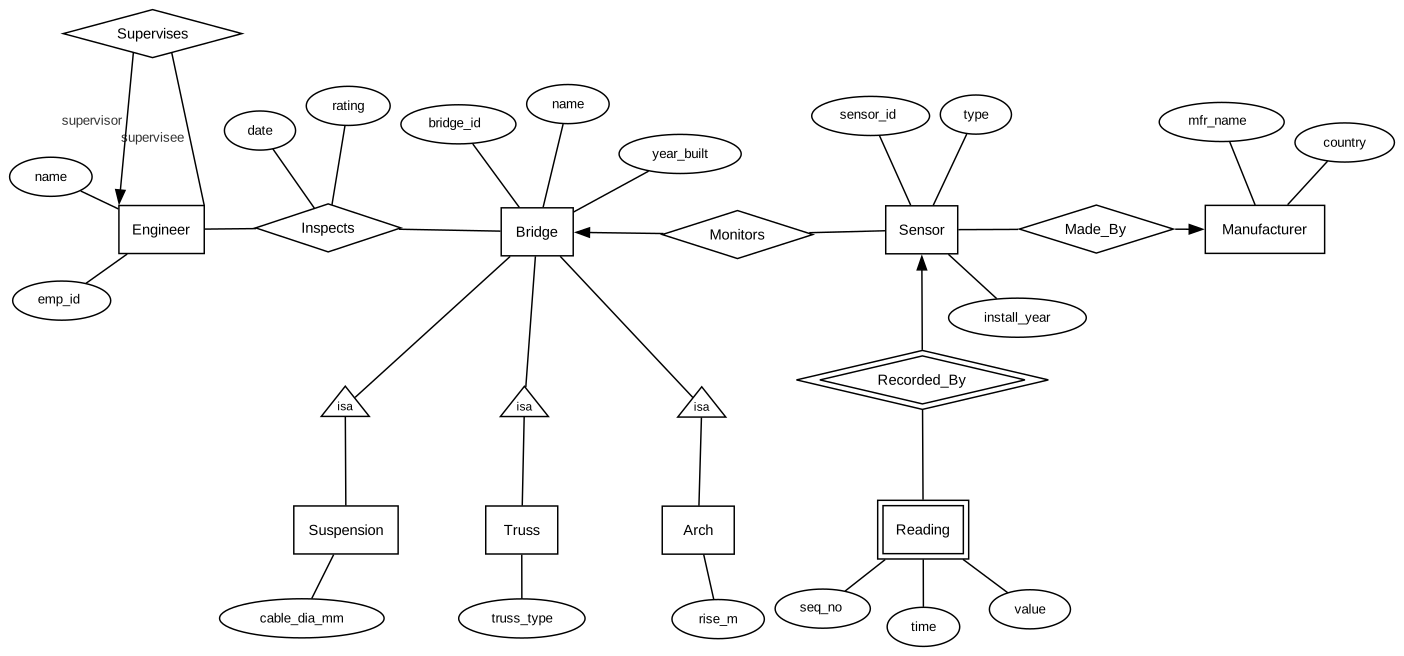
- Nouns with identity (bridge, sensor, manufacturer, engineer) became entity sets; properties (name, type, country) became attributes.
- “Monitors one bridge” and “made by one manufacturer” became many-one relationships with arrows. “Inspect bridges” became many-many.
- “Readings numbered from 1” is the signature of a weak entity set.
- “Reports to a supervisor, who is also an engineer” is a relationship of Engineer with itself, which needs roles; the arrow on the supervisor edge says each engineer has at most one supervisor.
- “Some bridges are suspension, truss, or arch bridges” is a subclass hierarchy.
- The diagram keeps
Inspectsas a relationship with attributes, which records only the latest inspection per engineer and bridge; the concept check in Section 10.3.3 shows how to change that if the history matters, and a real program would.
Two principles from Garcia-Molina et al. guide every choice: be faithful to the real world (a relationship’s multiplicity must match the program’s actual policy), and say everything once (a sensor’s bridge is recorded by Monitors, so it must not also be typed into a bridge_name attribute of Sensor, where the two copies could drift apart).
TipActive Learning: A pressure-monitoring network
Work in pairs, ten minutes. Draw an E/R diagram for these requirements, then compare with the pair next to you.
A water utility monitors its distribution network. Junctions have an ID and an elevation; some junctions are hydrants, which also have a flow rating. Pipes have an asset number, a diameter, a material, and an installation year, and each pipe runs from an upstream junction to a downstream junction. Pressure loggers, identified by serial number, are each installed at one junction. Each logger records readings numbered from 1, each with a time and a pressure. Maintenance crews make visits to pipes; each visit has a work-order number and a date.
NoteWhat to look for
- Pipe is tempting as a relationship between two junctions with roles upstream and downstream, and that is correct as far as it goes. But visits are made to pipes, so a pipe must be something a relationship can connect to: an entity set, with two many-one relationships to Junction playing the two roles.
- Hydrant is a subclass of Junction.
- Reading is a weak entity set supported by Logger.
- Visit is an ordinary entity set with key
work_order, many-one to Pipe; it is not weak, because the work-order number identifies it on its own. - The logger’s junction is many-one today; if loggers are moved and the utility wants to know where each reading was taken, the design needs installation periods, and the reading must be tied to them.
10.4 Set Theory for Data Management
An E/R diagram says what the data looks like but not what we can do with it. “Find the sensors that are due for calibration but not flagged as faulty” must have one precise meaning before a computer can answer it, and so must “bridges with no sensors.” Set theory supplies that meaning. Every entity set is a set of entities, every table will be a set of rows, and filtering, combining, and excluding records are set operations; Codd built the relational model on exactly this foundation (Codd 1970).
10.4.1 Sets, Subsets, and Cardinality
To reason about “all temperature sensors” as a single object, we need a vocabulary for collections that is unambiguous about what is in them. A set is a collection of distinct objects, its elements. Two properties matter for databases:
- a set has no order: \(\{S1, S2\}\) and \(\{S2, S1\}\) are the same set;
- a set has no duplicates: an element is either in the set or not, never in it twice.
We write \(x \in A\) for “\(x\) is an element of \(A\)” and \(x \notin A\) for its negation. A set is described either by listing its elements or, more usefully for queries, by a property its elements satisfy (set-builder notation): \[ A = \{x \in U \mid \text{condition on } x\}, \] read “the \(x\) in \(U\) such that the condition holds.” Here \(U\) is the universal set, everything under consideration; for our example, the six sensors in the city’s inventory, \[ U = \{S1, S2, S3, S4, S5, S6\}. \] The maintenance log defines two subsets of it: the sensors due for calibration, \(C = \{S1, S2, S6\}\), and the sensors flagged at the last data-quality check, \(F = \{S2, S5\}\). The set with no elements is the empty set, \(\emptyset\).
\(A\) is a subset of \(B\), written \(A \subseteq B\), if every element of \(A\) is also an element of \(B\); then \(B\) is a superset of \(A\). Both \(C \subseteq U\) and \(F \subseteq U\). Every set is a subset of itself, and \(\emptyset\) is a subset of every set. Do not confuse membership with inclusion: \(S2 \in F\) (an element belongs to a set), while \(\{S2\} \subseteq F\) (a one-element set is included in another).
The cardinality \(|A|\) is the number of elements of \(A\): \(|U| = 6\), \(|C| = 3\), \(|F| = 2\), \(|\emptyset| = 0\). If \(A \subseteq B\) then \(|A| \le |B|\). Counting queries (“how many sensors are flagged?”) are cardinalities.
10.4.2 Operations on Sets
Almost every question about an inventory combines two collections: due and flagged, due or flagged, due but not flagged. Five operations express these combinations. For sets \(A\) and \(B\) inside a universal set \(U\):
| Operation | Notation | Definition | With \(C\) and \(F\) |
|---|---|---|---|
| Union | \(A \cup B\) | \(\{x \mid x \in A \text{ or } x \in B\}\) | \(\{S1, S2, S5, S6\}\) |
| Intersection | \(A \cap B\) | \(\{x \mid x \in A \text{ and } x \in B\}\) | \(\{S2\}\) |
| Difference | \(A - B\) | \(\{x \mid x \in A \text{ and } x \notin B\}\) | \(C - F = \{S1, S6\}\) |
| Complement | \(A^c\) | \(\{x \in U \mid x \notin A\} = U - A\) | \(C^c = \{S3, S4, S5\}\) |
| Cartesian product | \(A \times B\) | \(\{(a, b) \mid a \in A \text{ and } b \in B\}\) | 6 ordered pairs |
A few remarks make these operations safe to use:
- The “or” of union is inclusive: \(S2\) is in both sets and appears once in the union, because sets have no duplicates.
- Difference is not symmetric: \(C - F = \{S1, S6\}\) are the sensors to calibrate that are otherwise fine, while \(F - C = \{S5\}\) is the flagged sensor that nobody has scheduled for calibration, which is probably the more urgent list.
- Difference goes by two symbols in the literature. Mathematics texts usually write \(A \setminus B\), which is also the symbol you will see in the lecture slides; database texts write \(A - B\) (Garcia-Molina et al. 2009, Ch. 2), and so does this book, because relational algebra’s difference (Section 10.6.4) uses the same sign. Both name exactly the same operation.
- The complement depends on the universal set. \(C^c\) within the sensor inventory is three sensors; within “all sensors the manufacturer ever made” it is millions.
- The Cartesian product is the odd one out: its elements are ordered pairs, so \((S1, S2) \ne (S2, S1)\) and \(A \times B \ne B \times A\) in general. Its size is \(|A \times B| = |A|\,|B|\). The product extends to any number of sets, \(A_1 \times A_2 \times \dots \times A_n\), whose elements are \(n\)-tuples. It is the operation that turns sets of values into sets of records, which is why it reappears at the heart of the relational model.
The widget below shades the region of a Venn diagram that each expression describes and lists its elements. Before selecting an expression, predict its elements; then check.
10.4.3 Properties of Set Operations
Two queries written differently can return the same answer, and a database system routinely rewrites the query you typed into an equivalent one that is faster to run. It may do so only because the operations obey algebraic laws, the same laws you use to rearrange arithmetic. For any sets \(A\), \(B\), \(C\) in a universal set \(U\):
- Commutative: \(A \cup B = B \cup A\) and \(A \cap B = B \cap A\). Difference and Cartesian product are not commutative.
- Associative: \((A \cup B) \cup C = A \cup (B \cup C)\) and likewise for \(\cap\), so \(A \cup B \cup C\) needs no parentheses.
- Distributive: \(A \cap (B \cup C) = (A \cap B) \cup (A \cap C)\) and \(A \cup (B \cap C) = (A \cup B) \cap (A \cup C)\).
- De Morgan’s laws: \((A \cup B)^c = A^c \cap B^c\) and \((A \cap B)^c = A^c \cup B^c\).
- Identities: \(A \cup \emptyset = A\), \(A \cap U = A\), \(A \cap \emptyset = \emptyset\), \(A - B = A \cap B^c\).
De Morgan’s laws are the ones that catch people. “Neither due nor flagged” is \((C \cup F)^c = C^c \cap F^c = \{S3, S4\}\); “not both due and flagged” is \((C \cap F)^c = C^c \cup F^c\), which is every sensor except \(S2\). The widget above lets you check both pairs: each pair shades the same region.
Two sets are disjoint if \(A \cap B = \emptyset\); then, and only then, \(|A \cup B| = |A| + |B|\). A collection of nonempty, pairwise disjoint subsets whose union is \(S\) is a partition of \(S\). Partitions are what a classification should be: if every bridge must be exactly one of suspension, truss, arch, or “other,” the four subclasses partition Bridge, and a query that counts bridges by type will add up to the total.
CautionConcept Check: Alerts on every bridge
Let \(H\) be the set of bridges with a high-strain alert this week and \(V\) those with a high-vibration alert. A dashboard should list the bridges that need no attention: no strain alert and no vibration alert. A colleague writes \(H^c \cup V^c\). Is that right?
TipAnswer
No. \(H^c \cup V^c = (H \cap V)^c\) is “not both alerts,” which includes a bridge with a strain alert only. The dashboard needs “neither,” \(H^c \cap V^c = (H \cup V)^c\). The mistake is De Morgan’s: negating an “or” turns it into an “and,” and negating an “and” turns it into an “or.”
10.4.4 Connecting Sets to ER Diagrams
The E/R diagram and the set notation describe the same system from two sides, and the link between them is what the relational model is built on:
- An entity set is a set: Bridge is the set of bridges, and each bridge is an element.
- A condition on attributes carves out a subset: \(\{b \in \text{Bridge} \mid b.\text{year\_built} < 1950\}\).
- A binary relationship is a subset of a Cartesian product: \(\text{Inspects} \subseteq \text{Engineer} \times \text{Bridge}\). The product contains every conceivable (engineer, bridge) pairing; the relationship set contains the ones that actually happened.
- Multiplicity is a property of that subset: Monitors is many-one from Sensor to Bridge exactly when no sensor appears in two of its pairs.
The last two points are worth rereading. A relationship is a set of tuples, and so, in a moment, will be every table.
10.5 The Relational Model
An E/R diagram is a design, not a database: it stores nothing and answers no queries, so it has to be turned into a structure a machine can hold. Before 1970, databases were navigational: a program found a sensor’s readings by following stored links from record to record, so every query was a small program, and changing how the data was linked broke the programs. Codd’s proposal (Codd 1970) was to store everything as tables and let users say what they want rather than how to reach it, leaving the “how” to the system. The relational model he defined became the basis of most database systems in use today, including SQLite, the one you are using in Assignment 2 (Garcia-Molina et al. 2009, Ch. 2).
10.5.1 Relations as Sets of Tuples
The relational model’s guarantees follow from definitions, not conventions, and the definition is one line of set theory. Given attributes \(A_1, \dots, A_n\) whose allowed values are the sets \(D_1, \dots, D_n\) (their domains), a relation \(R\) on those attributes is a subset of the Cartesian product of the domains: \[ R \subseteq D_1 \times D_2 \times \dots \times D_n . \tag{10.1}\] Each element of \(R\) is an \(n\)-tuple, one value per attribute. The product holds every conceivable combination of values; the relation holds the combinations that describe real things. Because a relation is a set:
- it has no duplicate tuples: a bridge cannot be stored twice;
- its tuples have no order: there is no “first bridge,” and a query must never rely on one;
- its values are atomic, one value per attribute per tuple, which is why the E/R model above insisted on atomic attributes.
Here is the Bridge relation of our monitoring program:
bridge_id, name, year_built, and length_m (a hypothetical inventory).
bridge_id |
name |
year_built |
length_m |
|---|---|---|---|
| B1 | Mill Creek Bridge | 1931 | 118 |
| B2 | Riverside Bridge | 1959 | 240 |
| B3 | Harbor Bridge | 1972 | 610 |
| B4 | Station Street Bridge | 1908 | 85 |
10.5.2 Relations, Tuples, Attributes, and Their Table Names
Textbooks say “relation” and “tuple”; practitioners and SQL say “table” and “row”. You need both vocabularies to read either, and they map one to one:
| Relational model | Table view | In Table 10.2 |
|---|---|---|
| relation | table | Bridge |
| tuple | row | (B3, Harbor Bridge, 1972, 610) |
| attribute | column | year_built |
| domain (type) | column type | integers |
| relation schema | table header | Bridge(bridge_id, name, year_built, length_m) |
The table picture is convenient and slightly misleading: a drawn table has a first row and a left-to-right order of columns, and a relation has neither. Attributes are identified by name, not position, and rows by their values. SQL departs from the set model in one visible way, which Lecture 10 will return to: a SQL table may hold duplicate rows unless you forbid them.
10.5.3 Domains, Keys, and Constraints
A bridge of negative length or two sensors with the same ID are errors the database can reject, but only if we tell it what is allowed. Each attribute has a domain, the set of values it may take: year_built an integer, length_m a positive real, type one of accelerometer, strain_gauge, temperature. A key of a relation is a set of attributes on which no two tuples may agree; the key chosen to identify tuples is the primary key, underlined in a schema:
Bridge(bridge_id, name, year_built, length_m)
Sensor(sensor_id, type, install_year, bridge_id)
The last attribute of Sensor refers to a bridge. A foreign key is an attribute (or set of attributes) of one relation whose values must appear as key values of another: every bridge_id in Sensor must be the bridge_id of some tuple in Bridge. In set notation, the constraint is an inclusion, \[
\pi_{\text{bridge\_id}}(\text{Sensor}) \subseteq \pi_{\text{bridge\_id}}(\text{Bridge}),
\] using the projection operator of Section 10.6.2. This is the referential-integrity constraint that the E/R arrow alone did not impose, and it is how a relational database prevents readings from being attached to a sensor, or a sensor to a bridge, that does not exist.
bridge_id is a foreign key into Bridge.
sensor_id |
type |
install_year |
bridge_id |
|---|---|---|---|
| S1 | accelerometer | 2019 | B1 |
| S2 | strain_gauge | 2019 | B1 |
| S3 | strain_gauge | 2021 | B2 |
| S4 | accelerometer | 2021 | B3 |
| S5 | temperature | 2022 | B3 |
| S6 | strain_gauge | 2022 | B3 |
10.5.4 Schema versus Instance
Installing a sensor on a new bridge changes the data but not the design; adding a column for each sensor’s calibration date changes the design. Confusing the two is a common source of muddled requirements. The schema of a database is its structure: the relations, their attributes, domains, keys, and other constraints. It changes rarely, by deliberate redesign. An instance is the set of tuples stored in each relation at one moment; it changes with every insertion, update, and deletion. Table 10.2 and Table 10.4 show one instance of the schema written above them.
Constraints belong to the schema, not to the instance. In today’s instance no two bridges share a name, but that does not make name a key; the instance might satisfy it by luck (Garcia-Molina et al. 2009, Ch. 4). A key is a promise about every instance the database will ever hold, and only the people who know the monitoring program can make it.
CautionConcept Check: Keys from one instance
In Table 10.4, is type a key of Sensor? Is the pair (bridge_id, type)?
TipAnswer
type is not: three tuples share strain_gauge. The pair (bridge_id, type) happens to be unique in this instance, but it is not a key, because nothing stops the city from putting a second accelerometer on the Harbor Bridge next year. Uniqueness in one instance is evidence, not a guarantee; keys are declared from knowledge of the world.
ImportantExercise
The city adds a sensor S7, a temperature sensor installed on bridge B4 in 2024, and removes S5.
Which of the following changed: the schema of Sensor, its instance, or both?
The city then decides to record each sensor’s calibration date. What changes now?
Someone tries to insert a sensor S8 on bridge B9. Which constraint rejects it?
TipSolution
Only the instance: one tuple inserted, one deleted, same attributes and constraints.
The schema: Sensor gains an attribute
calibration_date(with its domain, dates, and a decision on whether it may be missing). Every existing tuple of the instance must then be given a value or marked as missing.The foreign key from Sensor.
bridge_idto Bridge: B9 is not thebridge_idof any bridge, so the insertion would break \(\pi_{\text{bridge\_id}}(\text{Sensor}) \subseteq \pi_{\text{bridge\_id}}(\text{Bridge})\).
10.6 Relational Algebra
“Find the names of bridges that carry accelerometers” is clear to a person and ambiguous to a machine: which table, matched how, which columns returned? Relational algebra is a small set of operators that take relations as input and produce a relation as output (Garcia-Molina et al. 2009, Ch. 2). It plays the role for tables that arithmetic plays for numbers: a few operations, combined freely, express every question we will need, and the SQL of Lecture 10 is built on the same operations.
10.6.1 Queries Return Relations
If the result of a query were a different kind of object from its input, we could not feed one query into another. Every relational-algebra operator returns a relation; this property, closure, is what makes composition possible, exactly as the sum of two numbers is a number you can multiply. A query can therefore be written three ways that mean the same thing:
- in words: the names of bridges built before 1950;
- in relational algebra: \(\pi_{\text{name}}\big(\sigma_{\text{year\_built} < 1950}(\text{Bridge})\big)\);
- in SQL (Lecture 10):
SELECT name FROM Bridge WHERE year_built < 1950.
The operators come in two families: those that work on one relation’s rows or columns (select, project, rename), and those that combine two relations (products and joins, and the set operations union, difference, and intersection).
10.6.2 Select and Project
The two most common requests are “only these rows” and “only these columns.”
Selection \(\sigma_{C}(R)\) keeps the tuples of \(R\) that satisfy the condition \(C\), a comparison of attributes with constants or with each other, combined with and (\(\wedge\)), or (\(\vee\)), and not (\(\neg\)): \[ \sigma_{C}(R) = \{t \in R \mid C(t) \text{ is true}\}. \] It is set-builder notation, applied to a table. The result has the same schema as \(R\):
bridge_id |
name |
year_built |
length_m |
|---|---|---|---|
| B1 | Mill Creek Bridge | 1931 | 118 |
| B4 | Station Street Bridge | 1908 | 85 |
Projection \(\pi_{L}(R)\) keeps only the attributes in the list \(L\). Because the result is a set, any tuples that become identical are merged: projecting Sensor onto type gives three tuples, not six.
type |
|---|
| accelerometer |
| strain_gauge |
| temperature |
The widget applies a selection and then a projection to Sensor. Choose which types and installation years to keep and which attributes to show, and watch the row count: selection can only remove rows, and projection can remove more by merging duplicates.
10.6.3 Cross Product and Joins
What we know about one sensor lives partly in Sensor and partly in Bridge, and nearly every useful question needs both. The tool is a product followed by a filter.
The Cartesian product \(R \times S\) pairs every tuple of \(R\) with every tuple of \(S\); its schema is the attributes of both, with shared names qualified by their relation (Bridge.bridge_id, Sensor.bridge_id). With four bridges and six sensors, \(\text{Bridge} \times \text{Sensor}\) has \(4 \times 6 = 24\) tuples, most of them nonsense: the Station Street Bridge paired with a sensor on the Harbor Bridge. The product is rarely what we want, but it is the raw material of what we want.
A theta join \(R \bowtie_{C} S\) is a product followed by a selection, \[
R \bowtie_{C} S = \sigma_{C}(R \times S),
\] and the condition \(C\) keeps the pairs that belong together. With \(C\) the equality \(\text{Bridge.bridge\_id} = \text{Sensor.bridge\_id}\) we get each sensor alongside its own bridge, six tuples, with bridge_id appearing twice. The condition can be any comparison; for example, the sensors installed when their bridge was more than 50 years old: \[
\text{Bridge} \bowtie_{\text{Bridge.bridge\_id} = \text{Sensor.bridge\_id} \,\wedge\, \text{install\_year} - \text{year\_built} > 50} \text{Sensor}
\] returns S1 and S2 (installed at 88 years) and S3 (62 years), but not the Harbor Bridge’s sensors (49 and 50 years).
The natural join \(R \bowtie S\) is the join we want most often: it pairs tuples that agree on every attribute the two relations share by name, and keeps one copy of each shared attribute. Bridge and Sensor share bridge_id, so:
| bridge_id | name | year_built | length_m | sensor_id | type | install_year |
|---|---|---|---|---|---|---|
| B1 | Mill Creek Bridge | 1931 | 118 | S1 | accelerometer | 2019 |
| B1 | Mill Creek Bridge | 1931 | 118 | S2 | strain_gauge | 2019 |
| B2 | Riverside Bridge | 1959 | 240 | S3 | strain_gauge | 2021 |
| B3 | Harbor Bridge | 1972 | 610 | S4 | accelerometer | 2021 |
| B3 | Harbor Bridge | 1972 | 610 | S5 | temperature | 2022 |
| B3 | Harbor Bridge | 1972 | 610 | S6 | strain_gauge | 2022 |
Natural join is convenient and has one trap: it matches on every shared name. If Bridge and Sensor both had an attribute called name (the bridge’s name, the sensor’s model name), the natural join would silently demand that they be equal and return almost nothing. The cure is to rename one of them first (Section 10.6.5), or to use a theta join and say exactly what should match.
CautionConcept Check: The missing bridge
Why does the Station Street Bridge disappear from \(\text{Bridge} \bowtie \text{Sensor}\)? If a report must list every bridge with its sensors, including bridges that have none, is the natural join the right tool?
TipAnswer
A join is a selection on the product, and every tuple of the product is a pair of one bridge and one sensor. A bridge with no sensor is in no pair with a matching bridge_id, so it cannot survive. A report of every bridge needs an outer join, which keeps unmatched tuples and fills the missing side with nulls; it is not part of the core algebra, and Lecture 10 introduces it in SQL.
10.6.4 Union, Difference, and Intersection
Merging two maintenance lists, or finding bridges that have no sensors, are set questions asked of tables, and the set operations of Section 10.4.2 apply unchanged, with one requirement. \(R \cup S\), \(R - S\), and \(R \cap S\) are defined only when \(R\) and \(S\) have the same schema (the same attributes with the same domains): a list of sensor IDs cannot be unioned with a list of bridges. The two maintenance lists of Section 10.4.1, stored as relations Due(sensor_id) and Flagged(sensor_id), qualify:
- \(\text{Due} \cup \text{Flagged}\) is the four sensors needing any attention;
- \(\text{Due} \cap \text{Flagged} = \{S2\}\);
- \(\text{Flagged} - \text{Due} = \{S5\}\), the flagged sensor nobody has scheduled.
Difference is the operator for “no” and “never” questions. The bridges with no sensors are all bridge IDs minus those that occur in Sensor: \[ \pi_{\text{bridge\_id}}(\text{Bridge}) - \pi_{\text{bridge\_id}}(\text{Sensor}) = \{(\text{B4})\}. \] The projections are what make the two sides union-compatible. Intersection is not strictly necessary, since \(R \cap S = R - (R - S)\), but it is convenient.
10.6.5 Rename
To find pairs of sensors on the same bridge we must compare Sensor with itself, and two copies of one relation have the same attribute names, so a condition like “sensor_id < sensor_id” is meaningless. The rename operator \(\rho_{S(A_1, \dots, A_n)}(R)\) returns \(R\) with the relation called \(S\) and its attributes called \(A_1, \dots, A_n\); the short form \(\rho_{S}(R)\) renames only the relation, so its attributes can be written \(S.A\). With two renamed copies the self-join is ordinary: \[
\pi_{S1.\text{sensor\_id},\, S2.\text{sensor\_id},\, S1.\text{bridge\_id}}\Big(\sigma_{S1.\text{bridge\_id} = S2.\text{bridge\_id} \,\wedge\, S1.\text{sensor\_id} < S2.\text{sensor\_id}}\big(\rho_{S1}(\text{Sensor}) \times \rho_{S2}(\text{Sensor})\big)\Big)
\]
S1.sensor_id |
S2.sensor_id |
S1.bridge_id |
|---|---|---|
| S1 | S2 | B1 |
| S4 | S5 | B3 |
| S4 | S6 | B3 |
| S5 | S6 | B3 |
Rename has a second use: making schemas union-compatible when two sources name the same thing differently, such as a county list with attribute asset_no and the city’s with bridge_id.
10.6.6 Composing Operators
Real questions take several steps, and because every operator returns a relation, the output of one is the input of the next. “The names of bridges that carry accelerometers” is:
- \(\text{Accel} := \sigma_{\text{type} = \text{'accelerometer'}}(\text{Sensor})\), the accelerometers;
- \(\text{WithBridge} := \text{Bridge} \bowtie \text{Accel}\), each with its bridge;
- \(\text{Answer} := \pi_{\text{name}}(\text{WithBridge})\), just the names,
or, as one expression, \(\pi_{\text{name}}\big(\text{Bridge} \bowtie \sigma_{\text{type} = \text{'accelerometer'}}(\text{Sensor})\big)\), which returns the Mill Creek Bridge and the Harbor Bridge. The sequence of named steps is easier to write and to check; the single expression is what a database system manipulates. Because the operators obey algebraic laws like those of Section 10.4.3, the system is free to reorder the steps; selecting the accelerometers before joining, as above, touches far fewer tuples than joining first, and gives the same answer.
TipActive Learning: Predict the result
For each expression, write the result table on paper (or just its number of rows) before revealing it. The last three ask you to write the expression yourself.
10.7 From ER Diagrams to Relational Schemas
The design lives in a diagram and the data will live in tables, so we need a systematic way to get from one to the other without losing what the diagram says: which attributes identify what, which facts are many-one, which entities depend on others. The translation is nearly mechanical, and the rules below are those of Garcia-Molina, Ullman, and Widom (2009, secs. 4.5–4.6). We apply them to Figure 10.6 as we go.
10.7.1 Entity Sets Become Relations
The simplest construct gets the simplest rule: each (non-weak) entity set becomes a relation with the same attributes, and its key becomes the primary key.
Bridge(bridge_id, name, year_built)
Manufacturer(mfr_name, country)
Engineer(emp_id, name)
10.7.2 Relationships Become Foreign Keys or Junction Tables
A relationship has to be stored somewhere, and where depends on its multiplicity. The general rule: a relationship becomes a relation whose attributes are the keys of the entity sets it connects, plus the relationship’s own attributes. For the many-many Inspects:
Inspects(emp_id, bridge_id, date, rating)
Its key is the pair (emp_id, bridge_id), since the relationship set holds each pair at most once (the concept check in Section 10.3.3 again), and each of its two key attributes is a foreign key into the relation it came from. Such a relation is often called a junction table.
For a many-one relationship there is a better option. Monitors, many-one from Sensor to Bridge, would become Monitors(sensor_id, bridge_id) with key sensor_id alone, since each sensor appears once. It has the same key as Sensor, so the two can be combined into one relation, and the relationship becomes a foreign key on the “many” side:
Sensor(sensor_id, type, install_year, bridge_id, mfr_name)
Here bridge_id is a foreign key into Bridge and mfr_name one into Manufacturer, and the combination saves a join every time we ask where a sensor is. The same rule handles the self-relationship Supervises, many-one from supervisee to supervisor: Engineer gains a foreign key into Engineer itself, named for its role,
Engineer(emp_id, name, supervisor_id)
A one-one relationship is a special case of many-one, and the foreign key can go on either side. A many-many relationship can never be folded into an entity’s relation: a bridge has several inspecting engineers, and one attribute holds one value.
10.7.3 Weak Entity Sets and Composite Keys
A weak entity cannot be identified by its own attributes, so its relation must borrow identity from its owner. The relation for a weak entity set contains its own attributes plus the key attributes of the entity sets that support it, and its primary key is the combination:
Reading(sensor_id, seq_no, time, value)
sensor_id is at once part of the key and a foreign key into Sensor. The supporting relationship Recorded_By needs no relation of its own: everything it records is already in Reading.
10.7.4 Subclasses: Three Ways to Store an ISA Hierarchy
There is no single right way to store suspension, truss, and arch bridges, and the choice decides which queries are easy. Garcia-Molina et al. describe three strategies (Garcia-Molina et al. 2009, sec. 4.6):
- E/R style. One relation per entity set in the hierarchy, each holding the root’s key and that entity set’s own attributes: Bridge(bridge_id, name, year_built), Suspension(bridge_id, cable_dia_mm), Truss(bridge_id, truss_type), Arch(bridge_id, rise_m). Each subclass’s
bridge_idis a foreign key into Bridge. A question about all bridges reads one relation; the full description of a truss bridge needs a join. - Object-oriented. One relation for each subtree of the hierarchy that includes the root, that is, for each combination of classes an entity can belong to, holding all of that combination’s attributes: Bridge(bridge_id, name, year_built) for bridges of no special type, Truss(bridge_id, name, year_built, truss_type), and so on. Every bridge lives in exactly one relation; a question about all bridges needs a union.
- Null values. One relation with every attribute of the hierarchy, Bridge(bridge_id, name, year_built, cable_dia_mm, truss_type, rise_m), where attributes that do not apply hold the special value null. Nothing needs a join or a union, at the cost of many nulls and of the database no longer preventing a truss bridge from having a cable diameter.
For our program, where most questions (sensors, inspections) are about bridges in general and the structural attributes are consulted occasionally, the E/R style is the natural choice.
10.7.5 A Complete Translation
Applying the rules to every construct in Figure 10.6 gives the schema of the monitoring program, nine relations with their keys and foreign keys:
Bridge(bridge_id, name, year_built)
Suspension(bridge_id, cable_dia_mm); Truss(bridge_id, truss_type); Arch(bridge_id, rise_m)
Manufacturer(mfr_name, country)
Sensor(sensor_id, type, install_year, bridge_id, mfr_name)
Reading(sensor_id, seq_no, time, value)
Engineer(emp_id, name, supervisor_id)
Inspects(emp_id, bridge_id, date, rating)
| Foreign key | References | Came from |
|---|---|---|
Suspension.bridge_id, Truss.bridge_id, Arch.bridge_id |
Bridge | isa (E/R style) |
Sensor.bridge_id |
Bridge | Monitors (many-one) |
Sensor.mfr_name |
Manufacturer | Made_By (many-one) |
Reading.sensor_id |
Sensor | Recorded_By (weak entity set) |
Engineer.supervisor_id |
Engineer | Supervises (many-one, roles) |
Inspects.emp_id, Inspects.bridge_id |
Engineer, Bridge | Inspects (many-many) |
Every arrow, double border, and triangle of the diagram has become a key or a foreign key, and every question in Section 10.6 can now be asked of these tables. The engineer’s question from the start of the lecture (“which strain gauges on bridges built before 1950 have gone silent, and who inspected those bridges?”) is a join of Bridge, Sensor, Reading, and Inspects with a few selections, which you will be able to write in SQL after Lecture 10.
10.8 Putting It All Together
A monitoring program’s hardest questions are about relationships among its sensors, assets, readings, and people, and this lecture built the chain of tools that makes those relationships trustworthy. The E/R diagram fixes what the database must hold: entity sets, atomic attributes, keys, relationships with their multiplicities, weak entity sets for things numbered within other things, roles for entity sets related to themselves, and subclasses. Set theory gives every combination of records a precise meaning, with laws that let equivalent questions be recognized as equivalent. The relational model stores everything as relations, subsets of Cartesian products of domains, with keys and foreign keys that turn the diagram’s constraints into rules the database enforces. Relational algebra asks questions of those relations with six core operators, closed under composition. And the translation rules connect the design to the storage, construct by construct.
Lecture 10 writes the same schemas and queries in SQL, and Lecture 11 asks what makes one correct schema better than another. Assignment 2 puts the whole chain to work: you will design, implement, and query a database for a campus fleet of sensing kits, where every one of this lecture’s constructs has a natural place.
10.9 Exercises
In a building-energy audit, \(U\) is the set of 40 thermal zones of an office building, \(H\) the 12 zones whose heating valve was open at 3 AM last night, and \(W\) the 9 zones with a window contact reporting “open.” Five zones are in both \(H\) and \(W\).
How many zones are in \(H \cup W\), and how many in \((H \cup W)^c\)?
Write, in set notation, the zones heating with the window open, and the zones heating with the window closed.
Use a law from Section 10.4.3 to show that \(H - (H \cap W) = H - W\).
TipSolution
\(|H \cup W| = |H| + |W| - |H \cap W| = 12 + 9 - 5 = 16\); the complement has \(40 - 16 = 24\) zones. (Counting the intersection twice is exactly why \(|A \cup B| = |A| + |B|\) holds only for disjoint sets.)
Heating with the window open: \(H \cap W\) (5 zones). Heating with it closed: \(H - W = H \cap W^c\) (7 zones).
\(H - (H \cap W) = H \cap (H \cap W)^c = H \cap (H^c \cup W^c)\) by De Morgan, \(= (H \cap H^c) \cup (H \cap W^c)\) by distributivity, \(= \emptyset \cup (H \cap W^c) = H - W\).
- Read the following description of a traffic-signal monitoring system and name every entity set (with a key), attribute, relationship (with its multiplicity), weak entity set, role, and subclass it calls for. “Each signalized intersection, identified by a city node number, has one controller, identified by serial number. A controller runs timing plans numbered 1, 2, 3, … within that controller, each with a cycle length. Detectors, identified by serial number, are installed on approaches to an intersection; some detectors are cameras, which have a resolution, and some are inductive loops, which have a loop length. Corridors are coordinated sequences of intersections: each coordination link connects an upstream and a downstream intersection with an offset in seconds.”
TipSolution
Entity sets: Intersection (key node_id), Controller (key serial), Detector (key serial), TimingPlan (weak, partial key plan_no, attribute cycle_length). Relationships: Controls, one-one between Controller and Intersection (“has one controller,” and a controller serves one intersection); Runs, many-one from TimingPlan to Controller, the supporting relationship of the weak entity set; Installed_At, many-one from Detector to Intersection. Subclasses: Camera (resolution) and Loop (loop_length) isa Detector. Coordination: a relationship Links between Intersection and itself with roles upstream and downstream and the attribute offset_s. Whether it is many-many depends on the network; in a grid, an intersection is upstream of several others.
- Draw an E/R diagram for a structural-monitoring deployment in a multistory parking garage. The owner operates several garages, each with a name and address. Each garage has levels numbered 1, 2, 3, … and each level has bays labeled A, B, C, …. Tilt sensors and crack gauges, identified by serial number, are each mounted in one bay; crack gauges also have a gauge length. Each sensor records readings numbered from 1 with a time and a value. Engineers inspect levels, and each inspection has a date and a condition rating; a level can be inspected many times.
TipSolution
Garage is an ordinary entity set (key garage_id, or name if names are unique; attribute address). Level is weak, supported by Garage (partial key level_no), and Bay is weak, supported by Level (partial key bay_label), so a bay’s key is (garage_id, level_no, bay_label): a chain of weak entity sets, each numbered within the one above it. Sensor (key serial) is many-one to Bay; CrackGauge isa Sensor with gauge_length (TiltSensor may be a second subclass or simply the remaining sensors). Reading is weak, supported by Sensor. Because a level is inspected many times, Inspection is an entity set, not a relationship attribute: weak, supported by Engineer and by Level, with date in its key and rating as an attribute (or given its own inspection number as key).
The Sensor relation of Table 10.4 has schema Sensor(sensor_id, type, install_year, bridge_id).
Name the relation, its tuples, attributes, and domains in the vocabulary of tables.
Give a subset of attributes that is a key and a superset of it that is not a minimal key.
The city stores readings in Reading(sensor_id, seq_no, time, value). Write the referential-integrity constraint between Reading and Sensor as a set inclusion.
TipSolution
The Sensor table; its six rows; its four columns; the column types (text for
sensor_id,type, andbridge_id, integers forinstall_year).{
sensor_id} is a key. {sensor_id,type} also has distinct values on every pair of tuples, so no two tuples agree on it, but it is not minimal:typecan be removed and uniqueness remains. (Such a set is a superkey.)\(\pi_{\text{sensor\_id}}(\text{Reading}) \subseteq \pi_{\text{sensor\_id}}(\text{Sensor})\).
Using Bridge (Table 10.2) and Sensor (Table 10.4), write relational-algebra expressions for the following, and give each result.
The IDs of sensors on bridges longer than 200 m.
The IDs of bridges that have an accelerometer but no strain gauge.
The names of bridges carrying at least two sensors.
TipSolution
\(\pi_{\text{sensor\_id}}\big(\sigma_{\text{length\_m} > 200}(\text{Bridge} \bowtie \text{Sensor})\big) = \{S3, S4, S5, S6\}\).
\(\pi_{\text{bridge\_id}}(\sigma_{\text{type} = \text{'accelerometer'}}(\text{Sensor})) - \pi_{\text{bridge\_id}}(\sigma_{\text{type} = \text{'strain\_gauge'}}(\text{Sensor}))\). B1 has both, and B3 has an accelerometer and a strain gauge (S6), so the result is empty. An empty answer is a valid relation, and here it is the correct one.
Pair each sensor with a different sensor on the same bridge, as in Section 10.6.5, and keep the bridge: \(\pi_{\text{name}}\big(\text{Bridge} \bowtie \rho_{T(\text{bridge\_id})}(\pi_{S1.\text{bridge\_id}}(\sigma_{S1.\text{bridge\_id} = S2.\text{bridge\_id} \,\wedge\, S1.\text{sensor\_id} \neq S2.\text{sensor\_id}}(\rho_{S1}(\text{Sensor}) \times \rho_{S2}(\text{Sensor}))))\big)\) = {Mill Creek Bridge, Harbor Bridge}. The rename gives the projected attribute the name
bridge_idagain so that the natural join matches on it. Counting (“at least two”) is awkward in the core algebra; SQL’sGROUP BYandCOUNTin Lecture 10 make it one line.
- Translate your E/R diagram from Exercise 3 into a relational schema. Underline primary keys and list every foreign key with the relation it references.
TipSolution
For the design in the solution to Exercise 3:
- Garage(garage_id, name, address)
- Level(garage_id, level_no); FK
garage_id→ Garage - Bay(garage_id, level_no, bay_label); FK (
garage_id,level_no) → Level - Sensor(serial, kind, garage_id, level_no, bay_label); FK (
garage_id,level_no,bay_label) → Bay - CrackGauge(serial, gauge_length); FK
serial→ Sensor (E/R style) - Reading(serial, seq_no, time, value); FK
serial→ Sensor - Engineer(emp_id, name)
- Inspection(emp_id, garage_id, level_no, date, rating); FKs
emp_id→ Engineer and (garage_id,level_no) → Level
A foreign key into a relation with a composite key must itself be composite: a bay is referenced by all three of its key attributes, never by bay_label alone.
10.10 Additional Resources
- Codd’s paper introducing the relational model (Codd 1970) is readable after this lecture: its “relations,” “domains,” and “projection” are the ones defined here.
- Chen’s paper introducing the entity-relationship model (Chen 1976).
- The SQLite documentation on foreign keys shows how the constraints of Section 10.7 are declared and enforced in the database you use in Assignment 2 (note that SQLite enforces them only when
PRAGMA foreign_keys = ON).