Chapter setup: imports and shared names
import numpy as np
import matplotlib.pyplot as plt
import schemdraw
import schemdraw.elements as elmWe now know some of the physical principles behind how sensors (and transducers, generally) convert between physical stimuli and electrical signals (Lecture 2). We also know that electrical signals can be manipulated and massaged through circuits (Lecture 3). The main conceptual understanding of the two signal transformations (from physical stimuli to electrical signals, and from raw electrical signals to useful ones) was to think about these transformations as linear time-invariant systems represented by coupled ODEs, which we can analyze in the time and frequency domains. At the end, we get a useful electrical signal (most likely a voltage) that carries the information we need about the physical stimulus we’re measuring. Though analog signals are useful, one can derive more utility these days from a digital representation of them, since we can use our computing infrastructure to transmit, store, analyze and display this information virtually anywhere and however we want, at very little cost. This lecture builds the concepts needed to understand how that translation from analog to digital happens.
Every code block in this chapter assumes that the setup below has run first, in the same Python session: it imports the libraries and defines the names the blocks share (see About the code in the Welcome chapter).
import numpy as np
import matplotlib.pyplot as plt
import schemdraw
import schemdraw.elements as elmPicture someone locked inside the digital world — a homunculus in a box — whose only knowledge of the physical system outside comes through the measurements we hand over. The analog voltage arriving from Lecture 3’s circuits is continuous in two independent senses: it has a value at every instant of time, and that value can be any number within its range. A computer can afford neither. Its memory holds finitely many numbers, each with finitely many digits, so before the homunculus can see anything, the signal must be made discrete along both axes — and these two discretizations are different operations, with different names, different rules, and different ways of going wrong.
Discretizing time is called sampling: we keep the signal’s value only at selected instants and know nothing in between. Discretizing amplitude is called quantization: each kept value is rounded to the nearest of a finite set of levels. Only after both is the signal digital — a finite list of finite-precision numbers, which is the only thing that can cross into the box (Figure 5.1). The rest of this lecture takes the two operations in turn, asking of each the question that matters for measurement: what do we lose, and how do we keep the loss harmless?
t = np.linspace(0, 1, 1000)
x = 1.2*np.sin(2*np.pi*2*t) + 0.4*np.sin(2*np.pi*5*t + 1)
ts = np.arange(0, 1, 1/20); xs = 1.2*np.sin(2*np.pi*2*ts) + 0.4*np.sin(2*np.pi*5*ts + 1)
Q = 0.5; xq = np.round(x/Q)*Q; xsq = np.round(xs/Q)*Q
fig, axs = plt.subplots(2, 2, figsize=(7.0, 4.4), sharex=True, sharey=True)
axs[0,0].plot(t, x); axs[0,0].set_title("continuous (analog)", fontsize=9)
axs[0,1].stem(ts, xs, basefmt=" ", markerfmt="C0.", linefmt="C0-"); axs[0,1].set_title("discrete time (sampled)", fontsize=9)
axs[1,0].plot(t, xq, drawstyle="steps-post"); axs[1,0].set_title("discrete amplitude (quantized)", fontsize=9)
axs[1,1].stem(ts, xsq, basefmt=" ", markerfmt="C0.", linefmt="C0-"); axs[1,1].set_title("digital (both)", fontsize=9)
for ax in axs.flat: ax.set_yticks([])
axs[1,0].set_xlabel("time (s)"); axs[1,1].set_xlabel("time (s)")
plt.tight_layout(); plt.show()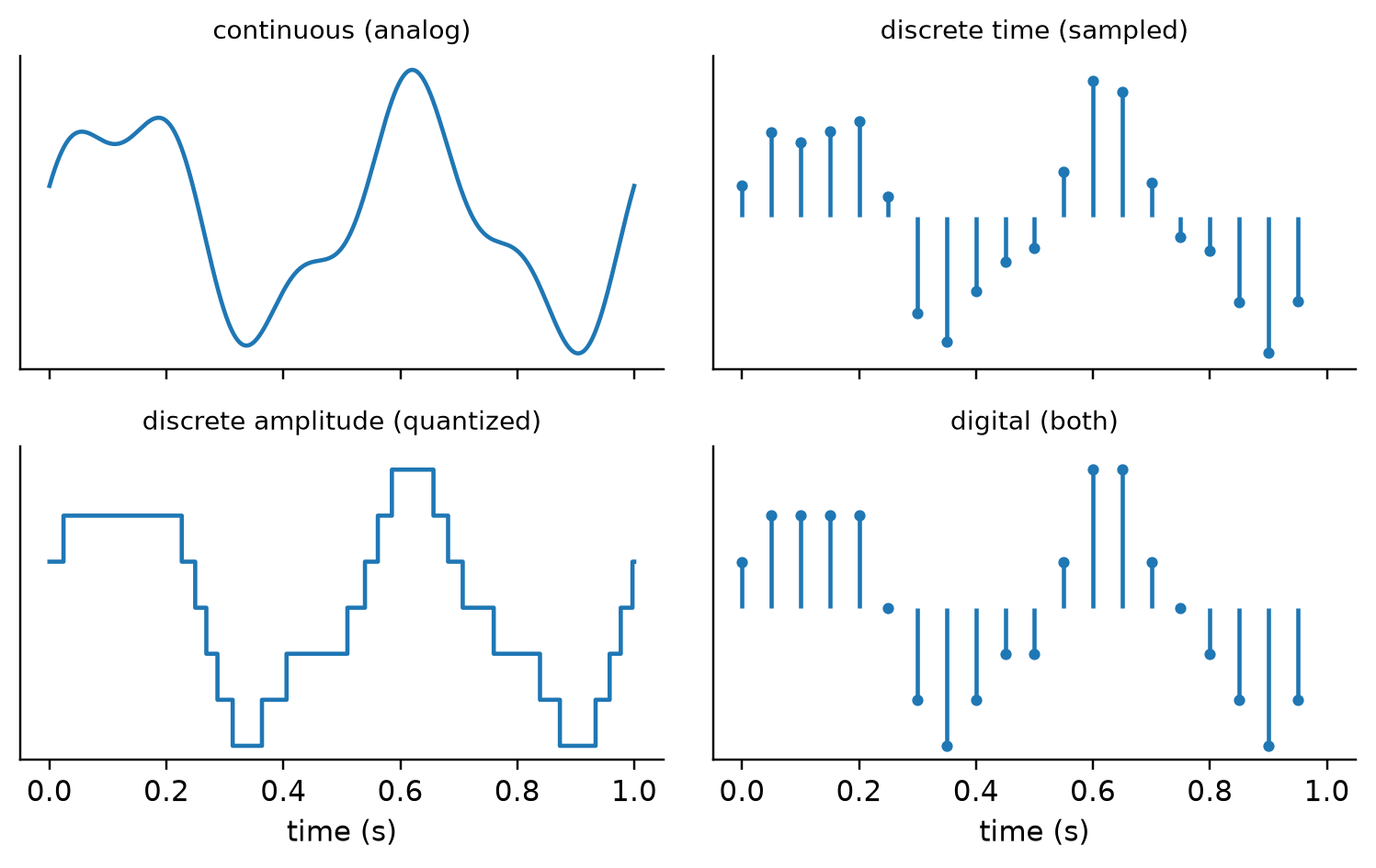
Suppose the homunculus can only glance out of its window every so often — snapshots, not a movie. In principle the snapshots could come at arbitrary instants, but nearly every real data-acquisition system takes them at equally spaced intervals \(\delta t\), because regular timing is easy to build and easy to reason about. The number of snapshots per second is the sample rate,
\[ f_s = \frac{1}{\delta t}, \tag{5.1}\]
measured in samples per second, or hertz (Figliola and Beasley 2019). The whole question of sampling is how large \(f_s\) must be for the snapshots to faithfully stand in for the movie — and the answer depends on how fast the signal itself wiggles, which requires a short but essential aside.
“How fast does the signal wiggle” is a vague phrase, and making it precise is one of the most useful ideas in all of engineering. Any signal we will care about can be regarded as a sum of sinusoids of different frequencies and amplitudes — a fact Lecture 6 develops properly — so alongside the familiar time-domain view (value versus time) every signal has a frequency-domain view: which frequencies it contains, and how strongly (Figure 5.2). The highest frequency present with meaningful amplitude, \(f_m\), is the number that captures “how fast it wiggles,” and it is the only property of the signal that sampling theory needs.
fig, (a1, a2) = plt.subplots(1, 2, figsize=(7.0, 2.8))
a1.plot(t, x); a1.set_xlabel("time (s)"); a1.set_ylabel("amplitude"); a1.set_title("time domain", fontsize=9)
a2.stem([2, 5], [1.2, 0.4], basefmt=" "); a2.set_xlim(0, 8); a2.set_ylim(0, 1.5)
a2.set_xlabel("frequency (Hz)"); a2.set_ylabel("amplitude"); a2.set_title("frequency domain", fontsize=9)
plt.tight_layout(); plt.show()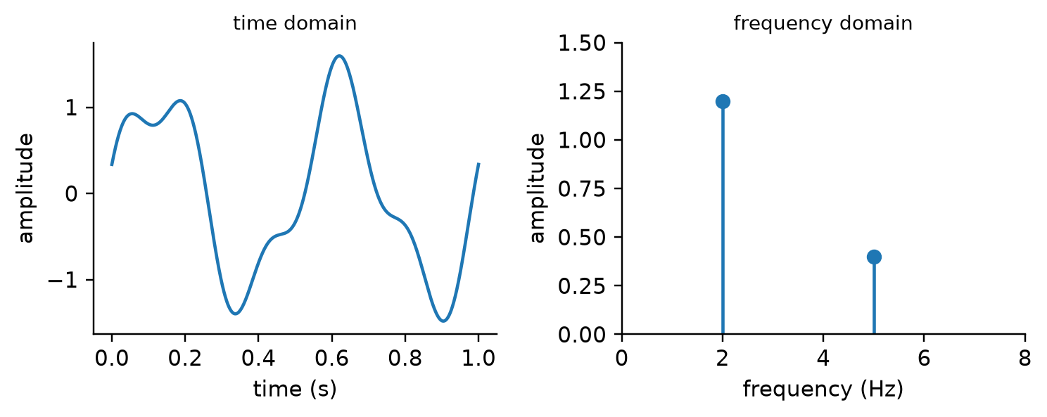
Glance out the window too rarely and the world can change completely between glances — a pendulum could swing any number of times while you looked away, and you would be none the wiser. The sampling theorem makes the intuition exact: to represent the frequency content of a signal whose highest frequency is \(f_m\), the sample rate must satisfy
\[ f_s > 2 f_m, \tag{5.2}\]
that is, more than two samples per period of the fastest component (Figliola and Beasley 2019). Half the sample rate, called the Nyquist frequency
\[ f_N = \frac{f_s}{2}, \tag{5.3}\]
is therefore the highest frequency a given sampling setup can honestly report. Two caveats keep the theorem honest in practice. It guarantees the frequencies are recoverable, not that the waveform will look right: for a faithful shape, practitioners sample at \(5 f_m\) to \(10 f_m\). And it assumes you actually know \(f_m\) — the interesting failure mode being what happens when you do not.
Here is the failure, and it is worse than mere blurriness: sample too slowly and a fast signal does not disappear — it impersonates a slower one. Figure 5.3 shows Figliola’s classic example: a 10 Hz sine sampled at \(f_s = 12\) Hz produces samples that fall exactly on a 2 Hz sine. The 10 Hz reality enters the data as a 2 Hz fiction, and nothing in the sampled record can tell you which one you have. This false identity is called an alias frequency (Figliola and Beasley 2019).
tt = np.linspace(0, 1, 2000)
f_sig, f_s = 10.0, 12.0
f_alias = abs(f_sig - f_s*round(f_sig/f_s))
tk = np.arange(0, 1, 1/f_s)
fig, ax = plt.subplots(figsize=(6.6, 3.0))
ax.plot(tt, np.sin(2*np.pi*f_sig*tt), color="0.75", lw=1, label="true signal, 10 Hz")
ax.plot(tt, np.sin(2*np.pi*(-f_alias)*tt), "C1--", lw=1.5, label=f"alias, {f_alias:g} Hz")
ax.plot(tk, np.sin(2*np.pi*f_sig*tk), "C0o", ms=5, label="samples at 12 Hz")
ax.set_xlabel("time (s)"); ax.set_ylabel("amplitude"); ax.legend(fontsize=8, loc="upper right")
plt.show()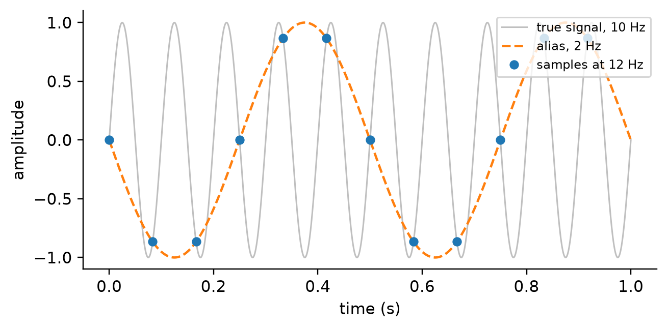
Which lower frequency does a too-fast signal impersonate? Every frequency above \(f_N\) is folded back into the interval \([0, f_N]\), mirror-fashion, about multiples of \(f_N\) — so the alias of any \(f\) is
\[ f_a = \left|\, f - f_s \cdot \mathrm{round}(f/f_s) \,\right|, \tag{5.4}\]
the distance from \(f\) to the nearest multiple of the sample rate. For the example: \(f = 10\) Hz, \(f_s = 12\) Hz, nearest multiple 12, \(f_a = 2\) Hz. The practical defenses are two, and you have already met the hardware for both: choose \(f_s\) comfortably above \(2 f_m\), and make sure nothing above \(f_N\) reaches the converter by placing a low-pass filter — Lecture 3’s RC circuit, promoted to the title of anti-aliasing filter — in front of it (Lecture 5 takes up its design). A structural-monitoring cautionary tale: log a bridge deck at 5 samples per second to “save storage,” and a 7 Hz mode dutifully appears in your data as a phantom 2 Hz mode — the kind of error no amount of downstream modeling can undo, because the data are not wrong, they are consistently wrong.
Build the intuition yourself: slide the signal frequency past the Nyquist frequency and watch the alias appear where the folding formula says it must.
Even with aliasing defeated, one subtlety remains, because a real record is finite: we sample for a total time \(N\,\delta t\) and then stop. The frequency-domain view built from \(N\) samples can only report content at discrete frequencies spaced
\[ \delta f = \frac{f_s}{N}, \tag{5.5}\]
apart — the frequency resolution of the record. If the record happens to hold a whole number of periods of the signal, its frequencies land exactly on that grid and the amplitudes come out true; if not, the record effectively truncates a period mid-swing, and the signal’s energy smears into neighboring frequencies — spurious content around the true spike known as leakage (Figure 5.4) (Figliola and Beasley 2019). The amplitude you read off can then be wrong even though nothing was aliased: that is the amplitude ambiguity of finite records. The cure is choosing the record length (or its \(\delta f\)) with the signal in mind — and, more generally, window functions that taper the record’s ends, which we take up with the DFT in Lecture 6.
fs_ = 1000.0
fig, axs = plt.subplots(1, 2, figsize=(7.0, 2.9), sharey=True)
for ax, periods in ((axs[0], 10.0), (axs[1], 9.5)):
    N = int(round(fs_ * periods / 100.0))
    tr = np.arange(N)/fs_
    X = np.abs(np.fft.rfft(np.sin(2*np.pi*100*tr)))/N*2
    fr = np.fft.rfftfreq(N, 1/fs_)
    ax.stem(fr, X, basefmt=" ", markerfmt="C0.", linefmt="C0-")
    ax.set_xlim(0, 250); ax.set_xlabel("frequency (Hz)")
    ax.set_title(f"{periods:g} periods in the record", fontsize=9)
axs[0].set_ylabel("amplitude")
plt.tight_layout(); plt.show()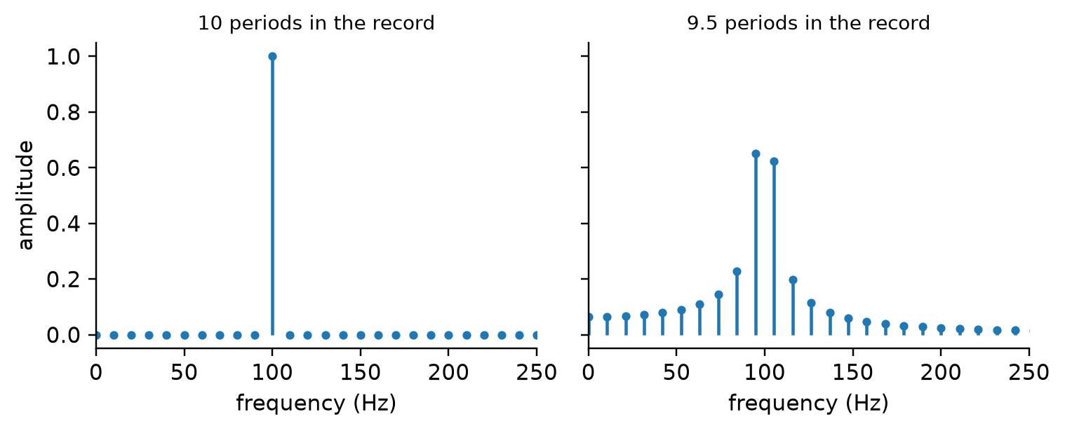
Back to the homunculus: even at the instants it does look out the window, suppose it can only describe what it sees as “dark,” “dim,” “bright,” or “very bright.” That is the second discretization — of the value itself — and it is forced on us by how computers store numbers.
Early machines stored information as holes punched in cards and paper tape — the player piano roll is the charming ancestor — and a hole admits exactly two states: there, or not there (Figliola and Beasley 2019). That two-state atom of information is the bit (a 1 or a 0), and an ordered sequence of \(M\) bits is a word, capable of \(2^M\) distinct patterns. Read as a base-2 number, an \(M\)-bit word counts from 0 to \(2^M - 1\): the 4-bit word 0101 is \(0\cdot8 + 1\cdot4 + 0\cdot2 + 1\cdot1 = 5\), an 8-bit word (a byte) reaches 255, a 16-bit word 65,535. The leftmost bit, weighing \(2^{M-1}\), is the most significant bit (MSB); the rightmost, weighing 1, the least significant bit (LSB) — vocabulary the converter section will need.
An analog-to-digital converter (ADC) accepts voltages over a full-scale range \(E_{FSR}\) (say, 0 to 3.3 V) and reports an \(M\)-bit word — so it can distinguish only \(2^M\) voltage levels, spaced
\[ Q = \frac{E_{FSR}}{2^M} \tag{5.6}\]
apart. That spacing is the converter’s resolution, the smallest voltage change guaranteed to move the output code — one LSB’s worth of input (Figliola and Beasley 2019). Every voltage between two levels gets rounded, and the rounding is the quantization error: with the usual half-step offset built into converters, at most
\[ e_Q = \pm\tfrac{1}{2} Q, \tag{5.7}\]
behaving like a small noise added to every sample (Figure 5.5). Two consequences deserve numbers. First, the error is relative to the reading, so small signals suffer most: on a 0–10 V, 8-bit converter, a 100 mV signal carries up to ±19.5% quantization error, while the same signal on 12 bits carries ±1.2% — which is why matching the signal’s amplitude to the converter’s range (Lecture 5’s amplifier, once more) matters as much as adding bits. Second, quantization sets a ceiling on the achievable signal-to-noise ratio: each added bit halves \(Q\), improving the ratio of full-scale signal to quantization noise by a factor of 2 — about 6 dB per bit,
\[ \mathrm{SNR}(\mathrm{dB}) = 20 \log_{10} 2^M \approx 6.02\,M. \tag{5.8}\]
A running-example number to keep: the ADXL335 (300 mV/g) read by a typical microcontroller’s 12-bit, 3.3 V converter gives \(Q = 3.3/4096 = 0.81\) mV — about 2.7 milli-g per count. No amount of averaging in the DATA third will resolve a 1 mg vibration from that record.
M = 3; FSR = 2.0; Qq = FSR/2**M
vin = np.linspace(-1, 1, 1000)
code = np.clip(np.round(vin/Qq), -(2**(M-1)), 2**(M-1)-1)
vq = code*Qq
fig, (a1, a2) = plt.subplots(1, 2, figsize=(7.0, 2.9))
a1.plot(vin, vq, drawstyle="steps-mid"); a1.plot(vin, vin, "k--", lw=0.8)
a1.set_xlabel("analog input (V)"); a1.set_ylabel("quantized output (V)"); a1.set_title(f"{M}-bit staircase, Q = {Qq:.2f} V", fontsize=9)
sig = 0.7*np.sin(2*np.pi*1.5*tt)   # stays inside the top code: quantization only, no saturation
sq = np.clip(np.round(sig/Qq), -(2**(M-1)), 2**(M-1)-1)*Qq
a2.plot(tt, sig, color="0.7", lw=1, label="input")
a2.plot(tt, sq, "C0", drawstyle="steps-post", lw=1, label="quantized")
a2.plot(tt, sig-sq, "C3", lw=0.8, label="error")
a2.axhline(Qq/2, color="C3", ls=":", lw=0.8); a2.axhline(-Qq/2, color="C3", ls=":", lw=0.8)
a2.set_xlabel("time (s)"); a2.legend(fontsize=7, loc="lower left"); a2.set_title("a sine, quantized", fontsize=9)
plt.tight_layout(); plt.show()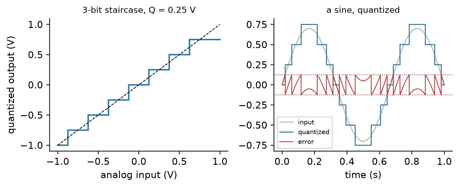
Slide the bit depth and watch both the staircase and the error shrink — each bit doubles the levels and buys ~6 dB.
This aside is optional — nothing later in the course depends on it. Read on if the staircase picture left you wondering how a one-bit converter could ever be useful, or what the “24-bit” label on a seismic recorder actually names.
By the staircase logic of Figure 5.5, a one-bit converter should be a joke: two levels, a resolution \(Q\) spanning half the range, a 6 dB signal-to-noise ceiling by Equation 5.8. Worse, the staircase we drew cannot even be built with one bit — rounding onto two’s-complement codes leaves reconstruction levels at \(-E_{FSR}/2\) and \(0\), with no code left over for “positive.” A real one-bit quantizer is nothing but a comparator — a circuit that answers a single question, is the input above mid-scale or below?, and one you will meet later in this lecture as the heart of the successive-approximation converter — reporting one of two symmetric levels: a mid-rise staircase, one step and no tread, and taken one sample at a time it is exactly as coarse as the arithmetic says.
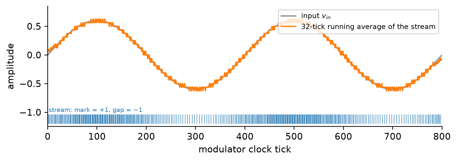
The rescue is to stop asking the comparator for the measurement and start asking it an easier question, very fast. A delta-sigma (\(\Delta\Sigma\)) modulator wraps the comparator in a feedback loop: each clock tick, the previous one-bit decision is subtracted from the input (the \(\Delta\)), the difference accumulates in an integrator (the \(\Sigma\)), and the comparator merely reports the accumulator’s sign. The feedback works to keep the accumulator near zero, which forces the density of highs in the output stream to track the input voltage — the homunculus never says more than “high” or “low,” but it says so millions of times a second, and the signal lives in the running average.
Averaging faster glances is worth something on its own — spreading the same quantization noise over a wider band buys about 3 dB, half a bit, per doubling of the rate — but the integrator is the real trick. Inside the loop, quantization error is suppressed where the integrator’s gain is large (low frequencies, where the signal lives) and shoved out to high frequencies where nothing of interest remains: noise shaping. A first-order loop turns each rate doubling into about 9 dB — one and a half bits — and higher-order loops climb steeper still (Schreier and Temes 2005). A digital low-pass filter then discards the out-of-band noise and decimates, handing back many-bit samples at a modest rate.
That is what sits behind the “24-bit” label on seismic recorders and load-cell electronics: a comparator clocked thousands of times faster than the signal band, a loop that shapes its error out of that band, and a filter that trades the surplus rate back for bits. The price is the trade itself — resolution is bought with oversampling — so delta-sigma owns the high-resolution, low-bandwidth corner where structural and geotechnical monitoring live, while the successive-approximation converter you will meet later in this lecture keeps the moderate-resolution, faster, multiplexer-friendly corner (a \(\Delta\Sigma\)’s digital filter has memory, so hopping between multiplexed channels means waiting for it to flush at every switch).
import schemdraw.dsp as dsp
with schemdraw.Drawing(show=False) as d:
    d += elm.Line().right().length(0.7).label('$v_{in}$', loc='left')
    d += (sm := dsp.Sum().right())
    d += dsp.Arrow().right().at(sm.E).length(0.9)
    d += (integ := dsp.Box(w=1.7, h=1.0).label('integrator'))
    d += dsp.Arrow().right().at(integ.E).length(0.9)
    d += (cmp := dsp.Box(w=2.0, h=1.0).label('comparator\n(1-bit ADC)'))
    d += dsp.Line().right().at(cmp.E).length(0.8)
    d += (nd := dsp.Dot())
    d += dsp.Arrow().right().length(2.2).label('1-bit stream at $N f_s$',
                                              loc='top', fontsize=8)
    d += (filt := dsp.Box(w=2.9, h=1.0)
                     .label('digital low-pass\n+ decimate by $N$'))
    d += (dsp.Arrow().right().at(filt.E).length(1.0)
             .label('24-bit samples\nat $f_s$', loc='right', fontsize=9))
    cx, cy = nd.center[0] - 2.0, nd.center[1] - 1.6
    d += (dac := dsp.Box(w=1.5, h=0.8).right().at((cx, cy))
                    .anchor('center').label('1-bit DAC'))
    d += dsp.Line().down().at(nd.center).toy(cy)
    d += dsp.Arrow().left().tox(dac.E)
    d += dsp.Line().left().at(dac.W).tox(sm.S)
    d += dsp.Arrow().up().toy(sm.S)
    d += elm.Label().at((sm.W[0] - 0.25, sm.W[1] + 0.3)).label('$+$')
    d += elm.Label().at((sm.S[0] + 0.3, sm.S[1] - 0.3)).label('$-$')
    d += elm.Label().at((cmp.N[0], cmp.N[1] + 0.25)).label('clock $N f_s$', fontsize=9)
from IPython.display import display
display(d.draw())
Nt = 800; n_ds = np.arange(Nt)
x_ds = 0.6 * np.sin(2 * np.pi * 2 * n_ds / Nt)   # two cycles of a slow sine
v_ds, y_ds = 0.0, -1.0; ys_ds = np.zeros(Nt)
for k in range(Nt):                              # the loop of panel (a), tick by tick
    v_ds += x_ds[k] - y_ds
    y_ds = 1.0 if v_ds >= 0 else -1.0
    ys_ds[k] = y_ds
avg_ds = np.convolve(ys_ds, np.ones(32) / 32, mode="same")
fig, ax = plt.subplots(figsize=(7.2, 2.6))
ax.plot(n_ds, x_ds, color="0.6", lw=1.6, label="input $v_{in}$")
ax.plot(n_ds, avg_ds, color="C1", lw=1.4,
        label="32-tick running average of the stream")
ax.eventplot(n_ds[ys_ds > 0], lineoffsets=-1.12, linelengths=0.16,
             colors="C0", linewidths=0.5)
ax.text(2, -1.02, "stream: mark = +1, gap = −1", fontsize=7, color="C0",
        va="bottom")
ax.set_xlim(0, Nt); ax.set_ylim(-1.25, 0.85)
ax.set_xlabel("modulator clock tick"); ax.set_ylabel("amplitude")
ax.legend(fontsize=8, loc="upper right")
plt.tight_layout(); plt.show()
If this aside caught your interest, Wikipedia’s article on delta-sigma modulation is the natural next step: it has the block diagrams for higher-order loops, the noise-shaping derivation, and the history, including why one-bit converters ended up inside nearly every audio device you own.
A colleague’s strain record looks “steppy,” like a staircase riding the waveform. Another’s looks smooth but shows a slow oscillation that the structure cannot physically produce. Which discretization failed in each case, and which knob — sample rate or bit depth — fixes which?
The steppy record is starved of amplitude resolution: too few bits (or, just as often, a small signal using a sliver of the converter’s range — amplify first!). The impossible slow oscillation is an alias: the sample rate was too low for some fast content, which folded down below \(f_N\). More bits cannot fix aliasing, and faster sampling cannot fix quantization — the two discretizations fail independently, which is why Figure 5.1 has two axes.
Everything so far treats the ADC as a magic box that rounds and reports. Opening the box is worth a few pages — not for the electronics for its own sake, but because each internal block explains one limit you will meet on a datasheet. The full pipeline promised at the start of this lecture reads: sensor → signal conditioning → multiplexer → sample-and-hold → ADC — and we take the remaining blocks in that order.
A monitoring project rarely has one sensor, but a good ADC is the most expensive block in the logger, so nobody builds one per channel. The multiplexer is the economizing trick: an electrically controlled selector switch that connects the converter to one input channel at a time, sweeping through them in turns. The economics come with arithmetic attached — the converter’s sample rate is shared, so a 200 kS/s ADC multiplexed across 8 channels delivers at most 25 kS/s per channel, and it is that per-channel rate, not the headline number, that must clear the sampling theorem. The channels are also no longer sampled at the same instant, a skew that matters when you later correlate signals (the DATA third will meet this as a timestamp problem).
The multiplexer’s datasheet line “16 single-ended / 8 differential” hides a second decision this lecture owes you. In a single-ended measurement, each channel’s voltage is measured against the logger’s common ground — one wire per sensor, sixteen channels from sixteen inputs, perfectly adequate for large, ground-referenced signals like our voltage-divider outputs. In a differential measurement, the converter reads the difference between a pair of inputs, neither of which needs to sit at ground — which costs two inputs per channel (sixteen become eight) but buys exactly what small or floating signals need. The Wheatstone bridge of Lecture 3 is the canonical customer: its output is the difference between two midpoints, both sitting near half the supply, and only a differential input can read it directly. Differential inputs also reject common-mode interference — noise picked up equally by both leads of a long cable cancels in the subtraction — which is why the rule of thumb runs: single-ended for short leads and volts, differential for long leads, millivolts, and anything bridge-shaped.
A converter needs a finite time to do its work, and the input must not move while it works — like asking a portrait subject to hold still for the exposure. The sample-and-hold circuit does exactly what its name says: a fast switch briefly connects the input to a capacitor (Lecture 3’s element that remembers voltage), which then holds the value steady, buffered by a high-input-impedance amplifier, while the ADC digitizes it (Figure 5.7) (Figliola and Beasley 2019).
with schemdraw.Drawing(show=False) as d:
    d += elm.Line().right().length(0.8).label('$v_{in}$', loc='left')
    d += elm.Switch().right().label('sample', loc='top')
    d += (nd := elm.Dot())
    d.push()
    d += elm.Capacitor().down().label('$C_{hold}$', loc='left')
    d += elm.Ground()
    d.pop()
    d += elm.Line().right().length(0.9)
    d += (op := elm.Opamp(anchor='in2').right().scale(0.8))
    d += elm.Line().right().at(op.out).length(0.4)
    d += (no := elm.Dot())
    d += elm.Line().right().length(0.6).label('to ADC', loc='right')
    d += elm.Line().up().at(no.center).length(1.3)
    d += elm.Line().left().tox(op.in1)
    d += elm.Line().down().at((op.in1[0], no.center[1]+1.3)).toy(op.in1)
d.draw()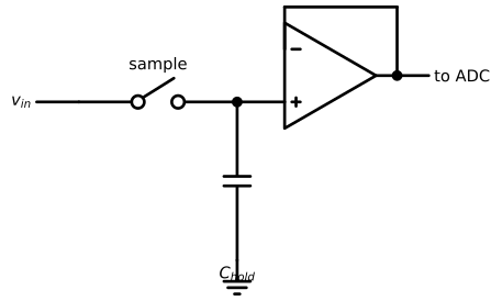
The triangle in Figure 5.7 is an operational amplifier, and this lecture borrows it twice on credit: as a follower (output equals input, but drawing almost no current from the source — Lecture 3’s loading medicine in one component) and as a comparator (output swings high or low according to which of its two inputs is larger — a one-bit answer to an analog question). How it does either is Lecture 5’s opening act; here it is enough that both behaviors exist and are cheap.
Strangely, the quickest route to building an analog-to-digital converter is to first build its opposite. A digital-to-analog converter (DAC) turns an \(M\)-bit word into a voltage, and Lecture 3 supplied all the parts: give each bit a resistor sized to its weight — \(R\) for the MSB, \(2R\), \(4R\), on to \(2^{M-1}R\) for the LSB — and let each 1-bit switch its resistor onto a common summing point feeding an op-amp (Figure 5.8). Each bit then contributes a current proportional to its binary weight, the currents add by KCL, and the output voltage is proportional to the word’s value \(X\):
\[ E_o \propto \frac{X}{2^M} \, E_{ref}, \tag{5.9}\]
a scaled replica of the number, in volts (Figliola and Beasley 2019).
with schemdraw.Drawing(show=False) as d:
    labels = ['$R$ (MSB)', '$2R$', '$4R$', '$8R$ (LSB)']
    for i, lab in enumerate(labels):
        y = -i*1.1
        d += elm.Line().right().length(0.7).at((0, y)).label('$b_%d$' % (3-i), loc='left')
        d += elm.Switch().right()
        d += elm.Resistor().right().label(lab, loc='top', fontsize=9)
        d += elm.Line().right().tox(6.6)
        if i > 0: d += elm.Line().up().toy(0)
    d += (nsum := elm.Dot().at((6.6, 0)))
    d += elm.Line().right().length(0.6)
    d += (op := elm.Opamp(anchor='in1').right().scale(0.8))
    d += elm.Line().down().at(op.in2).length(0.5)
    d += elm.Ground()
    d += elm.Line().right().at(op.out).length(0.3)
    d += (no := elm.Dot())
    d += elm.Line().right().length(0.5).label('$E_o$', loc='right')
    d += elm.Line().up().at(no.center).length(1.6)
    d += elm.Resistor().left().tox(nsum.center).label('$R_r$', loc='top', fontsize=9)
    d += elm.Line().down().toy(nsum.center)
d.draw()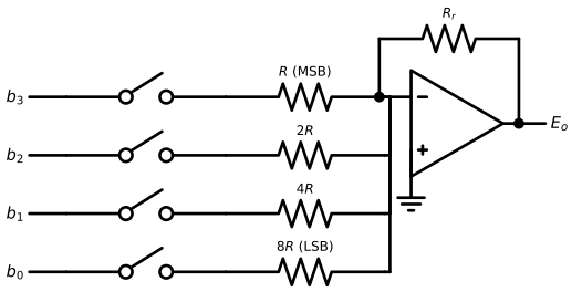
With a DAC, a comparator, and a sample-and-hold in hand, the most common ADC architecture nearly builds itself. The successive-approximation converter plays a game of twenty questions — or rather, \(M\) questions — with the held input voltage: set the MSB and ask the comparator “is my DAC’s output above the input?”; keep or clear the bit accordingly; repeat with the next bit down (Figliola and Beasley 2019). It is binary search, in silicon. Figure 5.9 traces Figliola’s example — a 4-bit, 0–15 V converter digitizing 10.1 V: trials at 7.5, 11.25, 9.375, and 10.3125 V settle on the code 1010, reported as 9.375 V, leaving a residual of 0.725 V. That is more than the \(\pm Q/2 = \pm 0.469\) V of Equation 5.7, and it should be: the bare search keeps a bit only when the trial stays at or below the input, so it always rounds down, and its error lies anywhere from 0 up to a full \(Q = 0.9375\) V. The half-step offset that real converters build in shifts every trial down by \(Q/2\); with it, the same input lands on 1011 = 10.3125 V, an error of 0.2125 V, back within \(\pm Q/2\). One clock tick per bit means a 12-bit conversion at a 1 MHz clock takes 12 µs — the origin of the sample-rate ceilings on converter datasheets. (Faster and slower siblings exist for other trade-offs: the flash converter answers all questions at once with \(2^M - 1\) comparators, and integrating converters trade speed for noise rejection in digital voltmeters.)
Ei, FSRs, Mb = 10.1, 15.0, 4
code_val, trials = 0, []
for b in range(Mb-1, -1, -1):
    trial = code_val + 2**b
    E_star = trial/2**Mb * FSRs
    trials.append(E_star)
    if E_star <= Ei: code_val = trial
E_final = code_val/2**Mb * FSRs
fig, ax = plt.subplots(figsize=(6.0, 3.0))
ax.axhline(Ei, color="0.4", ls="--", lw=1, label=f"input {Ei} V")
ax.step(range(1, Mb+1), trials, where="mid", color="C0", lw=1.5, label="DAC trial $E^*$")
ax.plot(range(1, Mb+1), trials, "C0o", ms=5)
for i, tv in enumerate(trials):
    ax.annotate(f"{tv:g}", (i+1, tv), xytext=(0, 7), textcoords="offset points", ha="center", fontsize=8)
ax.axhline(E_final, color="C2", ls=":", lw=1, label=f"final code 1010 → {E_final:g} V")
ax.set_xticks(range(1, Mb+1)); ax.set_xlabel("clock tick (bit under test, MSB first)"); ax.set_ylabel("voltage (V)")
ax.set_ylim(6, 12.5); ax.legend(fontsize=8, loc="lower right")
plt.show()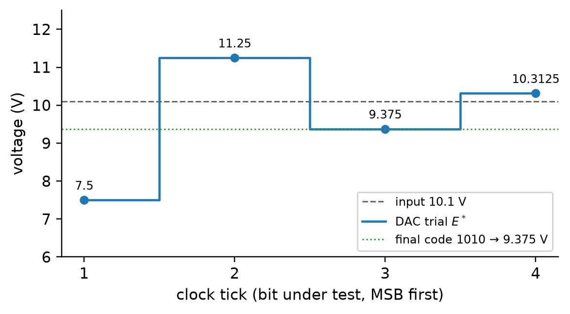
Find the ADC section of any microcontroller datasheet you can get your hands on (the Raspberry Pi Pico’s RP2040, for instance, whose ADC you will meet in the assignments). Identify: the bit depth and full-scale range (compute \(Q\)), the maximum sample rate (how many channels can it serve at 1 kHz each through its multiplexer?), and whether a sample-and-hold is mentioned. Every line should now map to a section of this lecture.
Digitization is two separate discretizations, each with its own failure mode and its own defense: sampling discretizes time (choose \(f_s > 2f_m\), filter out what lies above \(f_N\), and mind the finite record’s leakage), and quantization discretizes amplitude (choose bits and range so \(Q\) is small against the signal, knowing every bit buys about 6 dB). Around the converter sits a small supporting cast — multiplexer, sample-and-hold, op-amp, and a DAC running the successive-approximation search — that turns those two ideas into a working instrument. One more widening of the lens before we close. This lecture’s pipeline describes a single instrument, but most instruments you will meet today — including the ESP32-based wireless board you will use in the assignments — carry a radio and are designed to work as a collective: dozens of DAQ pipelines, each ending not in a display but in a transmission, joined into an IoT deployment or a wireless sensor network. What differentiates such systems is less the pipeline (which is exactly what you just learned) than the network architecture and the communication protocols and policies that coordinate it — and those bring their own constraints the single-instrument view never faced: a power budget when nodes live on batteries, a shared and limited wireless bandwidth, and the surprisingly hard problem of keeping distributed clocks synchronized well enough that samples from different nodes can be compared. The topic is far wider than we have time to treat here; for this course it is enough to recognize that every node in such a network is the pipeline of this lecture, plus a radio and a set of rules.
From here the signal is numbers, and numbers are where this course lives: Lecture 5 builds the analog conditioning that makes signals worth digitizing, Lecture 6 gives the frequency-domain view its full mathematical form, and the DATA third takes custody of everything the converter emits.
\(f_N = f_s/2 = 10\) Hz, so 12 Hz cannot be represented. By Equation 5.4 the nearest multiple of 20 Hz is 20, so \(f_a = |12 - 20| = 8\) Hz: a phantom 8 Hz mode. The theorem demands \(f_s > 24\) Hz; for waveform fidelity choose \(5\times\) to \(10\times\) the 12 Hz of interest — 60 to 120 Hz — and add an anti-aliasing filter with its cutoff near the chosen \(f_N\).
\(f_N = 50\) Hz. The 25 Hz component is below \(f_N\): it stays at 25 Hz. For 75 Hz, the nearest multiple of 100 is 100, so \(f_a = 25\) Hz; for 125 Hz, nearest multiple 100, \(f_a = 25\) Hz. All three components land on 25 Hz, superposing into a single spike whose amplitude is a phase-dependent mixture of the three — the record is not just missing information, it is confidently reporting a fiction.
12-bit: \(Q = 3.3/4096 = 0.81\) mV, or \(0.81/300 \times 10^3 = 2.7\) mg per count; SNR \(= 20\log_{10} 2^{12} \approx 72\) dB. 10-bit: \(Q = 3.3/1024 = 3.2\) mV \(= 10.7\) mg; SNR \(\approx 60\) dB. Whether 2.7 mg suffices depends on the application: ambient bridge vibration often lives below 10 mg, so the 10-bit mode would quantize the phenomenon of interest into two or three levels.
The 15th harmonic is 900 Hz (inside the CT’s band), so \(f_m = 900\) Hz and the theorem demands \(f_s > 1.8\) kHz; a practical choice is 5–10 kHz, with an anti-aliasing filter cutting off near \(f_s/2\). For bit depth: power computations square the waveform, so quantization error compounds; 12 bits (72 dB, 0.02% of full scale) is a common floor, and 16 bits (96 dB) is cheap insurance when small loads share a range sized for 75 A. The deeper lesson: the sensor’s bandwidth already truncates above 1 kHz, so sampling much beyond ~10 kHz buys nothing — the chain is only as wide as its narrowest link.
\(Q = 5/256 = 19.53\) mV. The search converges on \(\mathrm{round\,down}(3.7/Q) = 189 = \texttt{10111101}\), reported as \(189 \times 19.53\ \text{mV} = 3.691\) V — an error of 9 mV, within the \(Q\) bound. Eight bits at one tick per bit and 1 MHz: 8 µs. (Tracing the eight trials by hand — 2.5, 3.75, 3.125, 3.4375, 3.594, 3.672, 3.711, 3.691 V — is worth doing once in your life; the pattern of keep/clear decisions is the binary code.)