viewof text_input = Inputs.textarea({
  label: "Enter your text:",
  value: "Life, liberty and the pursuit of happiness.",
  rows: 2,
  width: "100%"
})9 Module 8: Data Representation and Compression
9.1 Module Overview
9.1.1 Learning Objectives
By the end of this module, students will be able to:
- Explain why different choices of how to represent (or compress) data/information offer tradeoffs that we should be aware of
- Predict the size of a simple ASCII text file based on its content
- Describe the differences between lossless and lossy compression schemes
- Understand the benefits of frequency domain representations for certain types of data
- Apply Huffman coding to an arbitrary text string
- Be aware of the compression algorithms used for JPEG and in other domains
9.1.2 Topics Covered
- Data Representation: understanding tradeoffs in representation choices
- Filesystems and ASCII encoding
- Types of data compression (lossless vs. lossy)
- Frequency Domain Representation of Data
- Huffman coding
- JPEG and other compression applications
- LLMs as compression algorithms?
9.1.3 Project Milestones
Schedule a meeting with the instructor for any clarifications needed before you go on Thanksgiving break.
9.2 Lecture Notes
9.2.1 Why Talk About Data Compression?
The database systems we’ve been studying are largely the “at rest” destination for data in a longer pipeline. Roughly speaking, data is first acquired, then transmitted, and finally stored. At each stage, size matters:
- The more data we transmit, the higher the bandwidth costs and the longer the transfer times
- The more data we store, the higher the storage costs and the slower our queries
Data compression allows us to represent, transmit, and store data in a more compact form. We measure file sizes in bits (or bytes, where 1 byte = 8 bits), and we quantify compression efficiency using the compression ratio—the ratio of the original size to the compressed size.
But before we can compress data, we need to understand how data is represented in the first place. Let’s start with something familiar: text.
9.2.1.1 How Text Becomes Bits: Character Encoding
When you save a text file, each character must be converted to a sequence of bits. The mapping from characters to bit sequences is called a character encoding. Different encodings make different tradeoffs:
ASCII (American Standard Code for Information Interchange):
- Uses exactly 7 bits per character (often stored as 8 bits for convenience)
- Can represent 128 characters: uppercase and lowercase English letters, digits, punctuation, and control characters
- Simple and compact for English text, but cannot represent characters from other languages
UTF-8 (Unicode Transformation Format - 8 bit):
- Variable-length encoding: 1 to 4 bytes per character
- ASCII characters use just 1 byte (backward compatible with ASCII)
- Extended characters (accents, non-Latin scripts, emoji) use 2-4 bytes
- The dominant encoding on the web today
UTF-16:
- Uses 2 or 4 bytes per character
- More efficient for texts with many non-ASCII characters (like Chinese or Japanese)
- Less efficient for English text compared to UTF-8
9.2.1.2 A Concrete Example
Consider the text: “Life, liberty and the pursuit of happiness.”
This string has 43 characters (including spaces and punctuation). How much storage does it require?
| Encoding | Bytes per Character | Total Size |
|---|---|---|
| ASCII | 1 byte (for these characters) | 43 bytes = 344 bits |
| UTF-8 | 1 byte (all ASCII characters) | 43 bytes = 344 bits |
| UTF-16 | 2 bytes minimum | 86 bytes = 688 bits |
| UTF-32 | 4 bytes fixed | 172 bytes = 1,376 bits |
For this English text, ASCII and UTF-8 are equally efficient. But if we included an emoji like 😊, UTF-8 would need 4 extra bytes for that single character, while ASCII couldn’t represent it at all.
9.2.1.3 Try It Yourself
Use the interactive tool below to explore how different text strings are encoded. Try entering text with special characters or emoji to see how the encoding affects file size:
This simple example illustrates a key insight: the same information can be represented in different ways, with different storage costs. This is the foundation of data compression—finding more efficient representations.
9.2.2 Change of Basis to Uncover Structure
Character encoding showed us that the same text can be represented with different numbers of bits. But there’s a deeper idea: sometimes changing your perspective on data reveals structure that wasn’t obvious before—structure that enables compression.
Consider a musical note. In the time domain, we represent it as a sequence of air pressure measurements over time—thousands of samples per second. But in the frequency domain, that same note might be described by just a few numbers: a fundamental frequency (the pitch) and a handful of harmonics with their amplitudes. The same information, radically different representations.
The mathematical tool that converts between these perspectives is the Fourier Transform (or its discrete version, the DFT/FFT). Here’s the key insight:
- Time-domain and frequency-domain representations contain exactly the same information
- They use the same number of values (no compression yet!)
- But frequency-domain representations often reveal that only a few components carry most of the signal’s energy
This is why frequency-domain analysis underlies many compression algorithms: once you see that most coefficients are near zero, you can throw them away.
9.2.2.1 Example: Accelerometer Data from a Building
Let’s look at real data. In Assignment 1, we analyzed accelerometer recordings from a building during an earthquake. The data was recorded at 100 Hz (one sample every 0.01 seconds) for 50 seconds—that’s 5,000 samples per sensor.
Here’s what one sensor’s data looks like in the time domain versus the frequency domain:
import numpy as np
import matplotlib.pyplot as plt

# Load the seismic response data
data = np.loadtxt('../../assignments/1/SeismicResponse.txt')
sensor_data = data[:, 0]  # First accelerometer (a1)

# Time domain parameters
dt = 0.01  # sampling period in seconds
n_samples = len(sensor_data)
time = np.arange(n_samples) * dt

# Compute FFT
fft_result = np.fft.fft(sensor_data)
frequencies = np.fft.fftfreq(n_samples, dt)

# Only take positive frequencies (signal is real)
pos_mask = frequencies >= 0
pos_frequencies = frequencies[pos_mask]
pos_amplitude = np.abs(fft_result[pos_mask]) / n_samples * 2  # Normalize

# Create side-by-side plots
fig, axes = plt.subplots(1, 2, figsize=(12, 4))

# Time domain plot
axes[0].plot(time, sensor_data, linewidth=0.5)
axes[0].set_xlabel('Time (s)')
axes[0].set_ylabel('Acceleration (m/s²)')
axes[0].set_title('Time Domain: 5,000 samples')
axes[0].grid(True, alpha=0.3)

# Frequency domain plot
axes[1].plot(pos_frequencies, pos_amplitude, linewidth=0.5)
axes[1].set_xlabel('Frequency (Hz)')
axes[1].set_ylabel('Amplitude (m/s²)')
axes[1].set_title('Frequency Domain: also 5,000 values')
axes[1].set_xlim(0, 20)  # Focus on low frequencies where building modes are
axes[1].grid(True, alpha=0.3)

plt.tight_layout()
plt.show()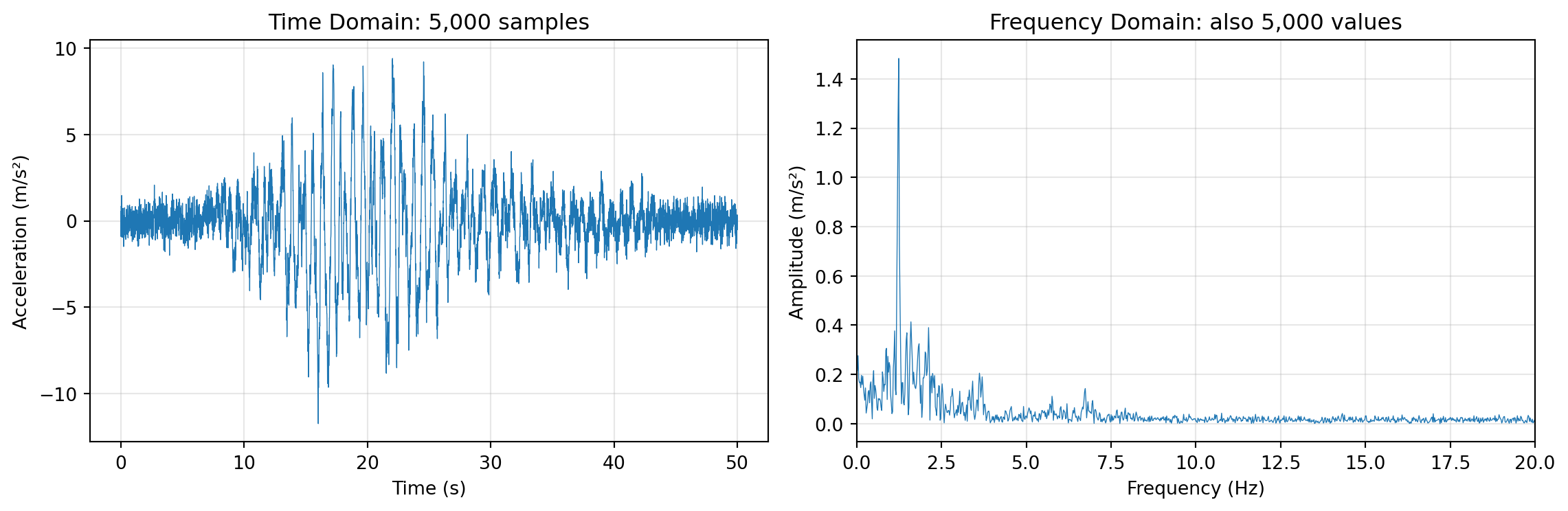
Notice something important in the frequency plot: most of the energy is concentrated in just a few frequency bands (the peaks). This is typical for structural vibration data—buildings have specific resonant frequencies (natural modes) that dominate the response.
9.2.2.2 From Representation to Compression
This observation suggests a compression strategy:
- Transform the signal to the frequency domain (using FFT)
- Identify the dominant peaks (frequencies with significant amplitude)
- Store only those frequency-amplitude pairs, discarding the rest
- To reconstruct, use the inverse FFT with only the kept components
For the signal above, instead of storing 5,000 time samples, we might store just 10-20 frequency-amplitude pairs—a compression ratio of 250:1 or better, with minimal loss of information relevant to structural analysis.
This approach works well when:
- The signal is composed of a few dominant frequencies (like building vibrations, musical notes, or periodic processes)
- The discarded components aren’t important for your application (e.g., high-frequency noise in structural monitoring)
9.2.3 Feature Extraction: A Different Kind of Compression
Sometimes you don’t need to preserve the full signal at all—you just need to extract specific features that answer your questions.
Consider sensor networks monitoring infrastructure. Most of the time, nothing interesting happens. Sensors might record data continuously, but transmitting and storing all of it would be expensive and wasteful. Instead, many systems use event-triggered approaches:
- Record data continuously in a local buffer
- Compute summary statistics (mean, standard deviation, peak value) over short windows
- Only transmit/store data when something unusual happens
For example, accelerometers monitoring seismic activity might:
- Compute the standard deviation of acceleration over 1-second windows
- If \(\sigma > 0.1 \text{ m/s}^2\), flag an event and transmit the raw data
- Otherwise, just store the summary statistics
This is feature extraction: we derive quantities that capture the essential characteristics of the data. The compression is extreme—instead of thousands of samples, we might store just a few numbers per time window. But this only works when we know in advance what features matter for our application.
The tradeoff is clear:
| Approach | Compression | Reconstructability | Use Case |
|---|---|---|---|
| Lossless (e.g., zip) | Moderate | Perfect | Archival, legal records |
| Frequency-domain | High | Approximate | Audio, images, signals |
| Feature extraction | Very high | None (features only) | Monitoring, anomaly detection |
9.2.4 Huffman Coding: Lossless Compression for Text
The previous sections discussed lossy compression—throwing away information we don’t need. But sometimes we need lossless compression: we want smaller files, but we must be able to reconstruct the original exactly. Huffman coding is a classic algorithm that achieves this for text (and other symbol sequences).
Let’s work through it with a concrete example: compressing the string “life liberty the pursuit of happiness” (37 characters).
9.2.4.1 Attempt 1: Fixed-Length Encoding
The simplest approach is to assign each unique character a fixed-length binary code. First, let’s identify the unique characters:
l, i, f, e, (space), b, r, t, y, h, p, u, s, o, a, nThat’s 16 unique characters. To represent 16 different values, we need \(\lceil \log_2(16) \rceil = 4\) bits per character.
| Character | Code | Character | Code |
|---|---|---|---|
| l | 0000 | h | 1000 |
| i | 0001 | p | 1001 |
| f | 0010 | u | 1010 |
| e | 0011 | s | 1011 |
| (space) | 0100 | o | 1100 |
| b | 0101 | a | 1101 |
| r | 0110 | n | 1110 |
| t | 0111 | y | 1111 |
Total size: 37 characters × 4 bits = 148 bits
This is already better than ASCII (which would use 37 × 8 = 296 bits), but can we do better?
9.2.4.2 Attempt 2: Variable-Length Encoding
Look at the character frequencies in our string:
| Character | Count | Character | Count |
|---|---|---|---|
| (space) | 5 | f | 2 |
| e | 4 | h | 2 |
| i | 4 | l | 2 |
| p | 3 | r | 2 |
| s | 3 | u | 2 |
| t | 3 | a | 1 |
| b | 1 | ||
| n | 1 | ||
| o | 1 | ||
| y | 1 |
Space appears 5 times, but ‘y’ appears only once. What if we used shorter codes for frequent characters and longer codes for rare ones? If space used only 2 bits instead of 4, we’d save 5 × 2 = 10 bits just from that one character!
But there’s a catch: with variable-length codes, how do we know where one code ends and the next begins? Consider if we assigned:
- space = 0
- e = 01
Then the sequence “01” could mean “space, something starting with 1” or just “e”. This ambiguity breaks decoding.
The solution is to use prefix-free codes: no code can be the beginning (prefix) of another code. For example:
- 0 and 01 are NOT both allowed (0 is a prefix of 01)
- 10 and 01 ARE both allowed (neither is a prefix of the other)
9.2.4.3 The Huffman Algorithm
David Huffman discovered an elegant algorithm that constructs the optimal prefix-free code for any character frequency distribution. Here’s how it works:
- Create a leaf node for each character, labeled with its frequency
- Build a tree by repeatedly:
- Find the two nodes with the smallest frequencies
- Create a new parent node with frequency = sum of the two children
- Remove the two children from the list, add the parent
- Repeat until only one node remains (the root)
- Assign codes by traversing the tree: left = 0, right = 1
Let’s apply this to our string. Starting with nodes sorted by frequency:
a:1, b:1, n:1, o:1, y:1, f:2, h:2, l:2, r:2, u:2, p:3, s:3, t:3, e:4, i:4, _:5(using _ for space)
Building the tree step by step:
- Combine a(1) + b(1) → node(2)
- Combine n(1) + o(1) → node(2)
- Combine y(1) + node(2) from step 1 → node(3)
- Continue combining the two smallest nodes at each step…
- Eventually all merge into a single root with frequency 37
The resulting Huffman tree produces these codes:
| Character | Huffman Code | Bits | Count | Total Bits |
|---|---|---|---|---|
| (space) | 101 | 3 | 5 | 15 |
| e | 001 | 3 | 4 | 12 |
| i | 000 | 3 | 4 | 12 |
| p | 1101 | 4 | 3 | 12 |
| s | 1110 | 4 | 3 | 12 |
| t | 1100 | 4 | 3 | 12 |
| f | 0100 | 4 | 2 | 8 |
| h | 0110 | 4 | 2 | 8 |
| r | 0101 | 4 | 2 | 8 |
| u | 0111 | 4 | 2 | 8 |
| l | 11111 | 5 | 2 | 10 |
| a | 10011 | 5 | 1 | 5 |
| b | 10000 | 5 | 1 | 5 |
| n | 11110 | 5 | 1 | 5 |
| o | 10010 | 5 | 1 | 5 |
| y | 10001 | 5 | 1 | 5 |
Total Huffman size: 142 bits
(Note: The exact codes depend on tie-breaking choices during tree construction. Different valid Huffman trees may produce slightly different codes, but all achieve the same optimal total bit count.)
9.2.4.4 Comparing Results
| Encoding | Bits | Compression vs ASCII |
|---|---|---|
| ASCII (8 bits/char) | 296 | — |
| Fixed 4-bit encoding | 148 | 50% |
| Huffman encoding | 142 | 52% |
Huffman coding saved 4% compared to fixed-length encoding, and 52% compared to ASCII!
The savings come from the principle: frequent characters get short codes, rare characters get long codes. The average code length is minimized.
9.2.4.5 Important Properties of Huffman Codes
- Prefix-free: No code is a prefix of another, so decoding is unambiguous
- Optimal: For a given frequency distribution, no prefix-free code uses fewer bits on average
- Requires the codebook: To decode, you need either the Huffman tree or the code table
The need to store/transmit the codebook is overhead that reduces the benefit for short messages. Huffman coding shines when:
- The message is long (codebook overhead is amortized)
- Character frequencies are skewed (some characters much more common than others)
- Lossless reconstruction is required
9.2.5 Other Compression Algorithms and Applications
We’ve covered the key concepts: character encoding, frequency-domain transformations, feature extraction, and Huffman coding. These ideas appear throughout the field of data compression. Here are a few more algorithms worth knowing about:
9.2.5.1 Run-Length Encoding (RLE)
Run-length encoding is perhaps the simplest compression algorithm. Instead of storing each symbol individually, RLE counts consecutive repetitions:
Original: BBWWWWBBBBBBWBBBBBBBBWW (23 characters)
RLE encoded: 2B4W6B1W8B2W (12 characters)
The encoding reads: “2 B’s, then 4 W’s, then 6 B’s, then 1 W, then 8 B’s, then 2 W’s.”
RLE works well when data has long runs of identical values—which is common in:
- Binary images (fax documents, simple graphics): Large regions of black or white
- Sparse data: Sensor readings that are mostly zero with occasional spikes
- Database columns: Sorted data where adjacent rows often have the same value
RLE performs poorly on data without repetition. For the string “abcdefgh”, RLE would produce “1a1b1c1d1e1f1g1h”—actually longer than the original!
9.2.5.2 JPEG Image Compression
JPEG is the dominant format for photographs, achieving 10:1 compression or better with minimal visible quality loss. It combines several techniques we’ve discussed:
Color space conversion: RGB colors are converted to YCbCr (luminance + chrominance). Human vision is more sensitive to brightness than color, so chrominance channels can be compressed more aggressively.
Block processing: The image is divided into 8×8 pixel blocks.
Discrete Cosine Transform (DCT): Each block is transformed to the frequency domain (similar to FFT, but using cosines). Low-frequency components represent smooth gradients; high-frequency components represent sharp edges and fine detail.
Quantization (the lossy step): DCT coefficients are divided by a quantization matrix and rounded. This discards high-frequency detail that humans don’t easily perceive. Higher compression = more aggressive quantization = more visible artifacts.
Entropy coding: The quantized coefficients are compressed using RLE (many coefficients become zero after quantization) and Huffman coding.
The “quality” setting in JPEG controls the quantization step—lower quality means more coefficients are rounded to zero, smaller files, but more visible blocking artifacts.
9.2.5.3 A Provocative Thought: LLMs as Compression?
Here’s an interesting perspective: language models like GPT or Claude can be viewed as compression algorithms.
Consider: a well-trained language model can predict the next word in a sentence with high accuracy. If you can predict what comes next, you don’t need to store it—you only need to store the surprises (the deviations from prediction).
This is exactly how modern compression algorithms like arithmetic coding work: they assign shorter codes to more predictable symbols. A language model that accurately predicts “the” after “in” can compress that sequence very efficiently.
In fact, researchers have shown that large language models achieve state-of-the-art compression ratios on text—they’re implicitly learning a very sophisticated model of language structure that enables extreme compression.
This connection between prediction and compression is deep: compression is prediction, and prediction is compression. The better you understand your data’s structure, the more efficiently you can represent it.