5 Module 4: Entity Relationship Diagrams and Set Theory
5.1 Module Overview
5.1.1 Learning Objectives
By the end of this module, students will be able to:
- Understand the structure and visual components of Entity Relationship Diagrams, and the motivation for using them
- Be able to distinguish between attributes, entity sets and relationships
- Be able to identify weak entity sets and how to display them
- Understand the need and use of roles and sub-classes in ER diagrams
- Recognize the value of set theory for describing and working with data records
- Be able to define sets in your own words, along with derivative terms such as sub-sets and super-sets
- Be able to apply (and recognize the notation for) the basic set operations of intersection, union, set difference, complement, cartesian product, cardinality
- Recognize the value of visual diagramming approaches to sets such as Venn diagrams, and identify equivalences between set theory expressions and their corresponding Venn diagrams
- Understand and be able to apply commutative, associative, distributive properties of set operations. Similarly, understand what are complimentary sets, and disjoint sets
5.1.2 Topics Covered
- Entity Relationship Diagrams (ER Diagrams)
- Components: attributes, entity sets, relationships
- Weak Entity Sets
- Roles and Subclasses in ER diagrams
- Set Theory
- Definition of sets, subsets, and supersets
- Basic operations: intersection, union, set difference, complement, cartesian product, cardinality
- Venn Diagrams
- Properties: commutative, associative, distributive, complementary sets, disjoint sets
5.1.3 Project Milestones
Come up with 3 ideas for your final project, regardless of whether or not you are already assigned to a team.
5.2 Lecture Notes
5.2.1 From Time Series to Data Structures
In Module 3, we focused on individual time series—sequences of measurements from sensors over time. We learned how to clean data, propagate uncertainty, detect outliers, and fit trends using linear regression. These techniques are essential for understanding what each sensor tells us.
But real engineering systems don’t consist of isolated sensors. Consider an environmental monitoring system for a watershed: you might have stream flow sensors at multiple locations, weather stations measuring precipitation and temperature, water quality sensors measuring pH and turbidity, and infrastructure sensors monitoring dams and bridges. Each sensor produces its own time series, but the real power comes from understanding the relationships among these measurements.
This raises new questions:
- How do we describe the structure of our data collection system itself?
- What entities (sensors, locations, infrastructure assets) exist in our system?
- How are these entities related to each other?
- What properties (attributes) does each entity have?
When systems become complex, with dozens or hundreds of sensors, multiple types of infrastructure, and intricate relationships, we need structured methods for organizing and visualizing this information. We can’t just keep track of it all in our heads or in ad-hoc spreadsheets.
Entity Relationship (ER) Diagrams provide a visual, intuitive way to model the structure of complex data systems before we implement them in databases. Think of ER diagrams as the architectural blueprint for your data—they help you think through what information you need to store and how different pieces relate to each other, long before you write a single line of database code.
5.2.2 Entity Relationship Diagrams
5.2.2.1 What Are Entity Relationship Diagrams?
Entity Relationship Diagrams (ER Diagrams) are graphical models that help us answer two fundamental questions about the data our system needs:
- What information must the database hold? (What entities and their properties exist?)
- What are the relationships among components of that information? (How do entities connect to each other?)
At their core, ER diagrams are visual representations where:
- Boxes (rectangles) represent collections of similar data elements (called entity sets)
- Arrows and diamonds represent connections and relationships between these elements
- Ovals represent properties (attributes) of the elements
ER diagrams serve as a crucial design tool—they’re typically the first step in database design. You sketch out an ER diagram to understand your data structure, then later translate it into a more rigorous model (like a relational database schema). The diagram helps you communicate with stakeholders, identify missing information, and catch design flaws early when they’re easy to fix.
Why are ER diagrams important?
- Communication: They provide a common visual language for engineers, database designers, and domain experts to discuss data structure
- Design validation: They help catch structural problems (missing entities, incorrect relationships) before implementation
- Documentation: They serve as living documentation of your system’s data architecture
- Foundation for implementation: They directly inform the design of relational databases and other data structures
5.2.2.2 A Simple Example: Infrastructure Monitoring System
Let’s start with a concrete example from civil engineering: a monitoring system for a set of bridges in a city.
The scenario: The city maintains several bridges and has installed sensors on each to monitor structural health. Each bridge has multiple sensors measuring different things (vibration, strain, deflection). We need to organize data about:
- The bridges themselves (location, construction year, type)
- The sensors (type, installation date, measurement units)
- The measurements collected over time
- Which sensors are installed on which bridges
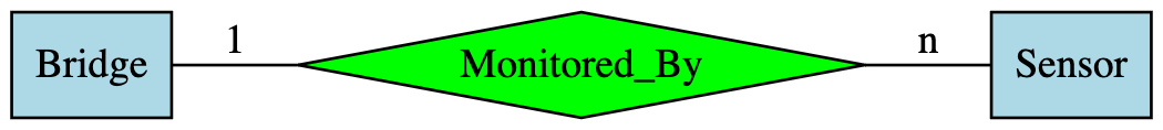
Here’s a simple ER diagram for this system:
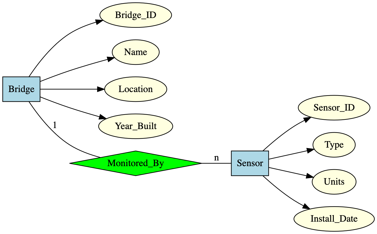
Reading this diagram:
- Bridge and Sensor (blue boxes) are entity sets—collections of bridges and sensors
- The ovals (yellow) attached to each box are attributes—properties that describe each entity
- The diamond (green) labeled “Monitored_By” represents a relationship between bridges and sensors
- The labels “1” and “n” indicate multiplicity: one bridge can be monitored by many (n) sensors
This simple diagram already tells us a lot: we can see at a glance what information we’re tracking and how bridges and sensors are related. As we develop our understanding, we’ll add more detail and handle more complex scenarios.
5.2.2.3 Basic Components of ER Diagrams
Now let’s examine each component of ER diagrams in detail, building up from the simplest concepts to more complex ones.
5.2.2.3.1 Entity Sets
An entity is an abstract object or “thing” that exists in the domain we’re modeling. Entities have distinct identity and properties that distinguish them from other objects.
Examples of entities:
- A specific bridge (e.g., the Roberto Clemente Bridge in Pittsburgh)
- A particular sensor (e.g., strain gauge #A-2301 installed on the bridge deck)
- A monitoring station (e.g., USGS stream gauge 03049500 on the Allegheny River)
- A maintenance event (e.g., the inspection performed on June 15, 2024)
An entity set is a collection (or group) of similar entities that share the same type and properties. Entity sets form the basis for database tables—each entity in the set will eventually become a row in a table.
Examples of entity sets:
- Bridge: The collection of all bridges in the city’s infrastructure system
- Sensor: The collection of all sensors deployed across the monitoring network
- MonitoringStation: All environmental monitoring stations in a watershed
- MaintenanceEvent: All recorded maintenance activities
Notation: Entity sets are represented as rectangles in ER diagrams.
Key insight: Think of entity sets as categories or types. Just as “Student” is a category containing individual students, “Bridge” is a category containing individual bridges. Each individual bridge is an entity; the collection of all bridges is the entity set.
5.2.2.3.2 Attributes
Attributes are properties or characteristics that describe the entities in an entity set. Each entity in a set has values for these attributes, and these values provide detailed information about that specific entity.
Notation: Attributes are represented as ovals connected to their entity set.
Example: The Bridge entity set might have these attributes:
Bridge_ID: A unique identifier for the bridgeName: The bridge’s name (e.g., “Fort Pitt Bridge”)Location: Geographic location or addressYear_Built: Construction yearBridge_Type: Type of bridge (suspension, truss, arch, etc.)Material: Construction materials usedLength: Span length in metersMax_Load: Maximum load capacity in tons
Types of Attributes:
ER diagrams distinguish several special types of attributes:
1. Key Attributes (Primary Keys)
Some attributes uniquely identify each entity in the set—no two entities can have the same value for these attributes. These are called key attributes or primary keys.
- In our Bridge example,
Bridge_IDwould be a key attribute - Each bridge has a unique ID; you can’t have two different bridges with the same ID
- Notation: Underline the attribute name in the oval (e.g., Bridge_ID)
2. Multi-valued Attributes
Some attributes can have multiple values for a single entity. For example:
- A bridge might be constructed from multiple materials (steel, concrete, and asphalt)
- A sensor might measure multiple quantities simultaneously
- A building might have multiple phone numbers
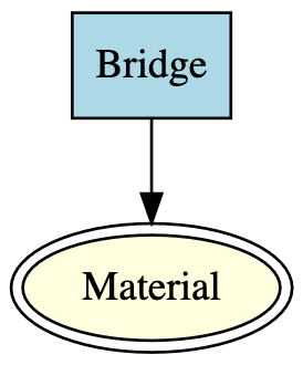
Notation: Multi-valued attributes are shown as double-lined ellipses (an ellipse within an ellipse).
Example: If the Material attribute of Bridge can hold multiple values, we’d draw it as:
3. Derived Attributes
Some attributes can be computed or derived from other existing attributes rather than stored directly. For example:
Ageof a bridge can be derived fromYear_Builtand the current yearAverage_Daily_Flowmight be derived from individual flow measurementsTotal_Sensorsfor a bridge could be counted from the relationship to the Sensor entity set
Notation: Derived attributes are shown as dashed-line ellipses.
Why distinguish derived attributes? It helps in database design—you typically don’t store derived values (they’re redundant and can become inconsistent), but you do want to document them in your ER diagram to show what information users can obtain.
Example diagram showing different attribute types:
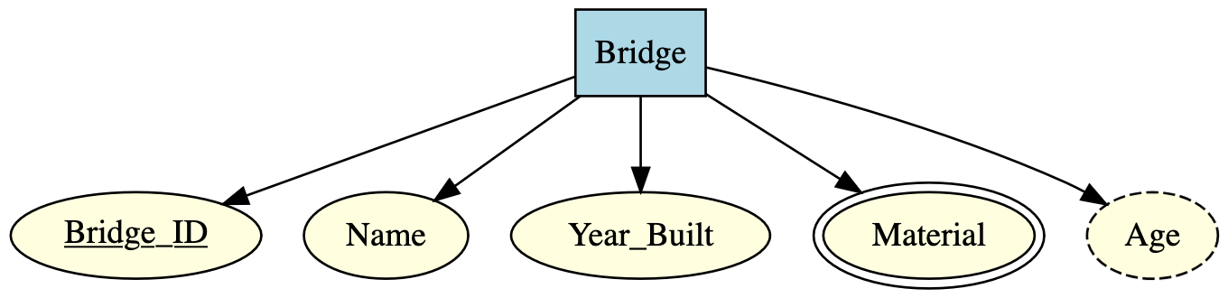
In this diagram:
Bridge_IDis underlined (key attribute)Materialhas double lines (multi-valued)Agehas dashed lines (derived fromYear_Built)
5.2.2.3.3 Relationships
Entity sets by themselves only tell us what things exist in our system. The real power of ER diagrams comes from modeling relationships—the connections among entity sets.
Definition: A relationship is a connection or association among two or more entity sets. Relationships capture how entities interact with, depend on, or relate to each other.
Notation: Relationships are represented as diamonds in ER diagrams, with lines connecting the diamond to the participating entity sets.
Examples from infrastructure monitoring:
- A Bridge is Monitored_By Sensors
- A Sensor Records Measurements
- A MaintenanceEvent Performed_On a Bridge
- An Engineer Inspects a Bridge
Multiplicity (Cardinality) of Relationships
A critical aspect of relationships is their multiplicity or cardinality—how many entities from each set can participate in the relationship. Understanding multiplicity is essential for correct database design.
For binary relationships (relationships between two entity sets), there are four common patterns:
1. One-to-One (1:1)
Each entity in set A is associated with at most one entity in set B, and vice versa.
Example: In a city management system, each Building has exactly one TaxRecord, and each TaxRecord belongs to exactly one Building.
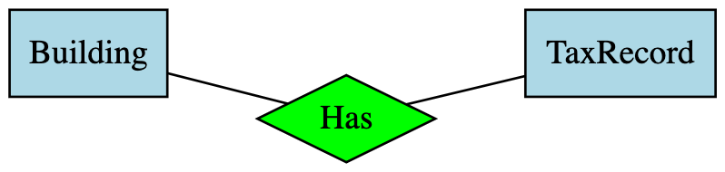
Notation: Arrow pointing to both entity sets, or labels “1” on both sides.
2. One-to-Many (1:n)
Each entity in set A can be associated with multiple entities in set B, but each entity in B is associated with at most one entity in A.
Example: One Bridge is monitored by many Sensors, but each Sensor is installed on only one Bridge.
Notation: Arrow points toward the “one” side, or labels “1” and “n” on the respective sides.
3. Many-to-One (n:1)
This is the reverse of one-to-many: multiple entities in set A can be associated with a single entity in set B.
Example: Many Sensors are manufactured by one Manufacturer, but each Manufacturer produces many sensors.
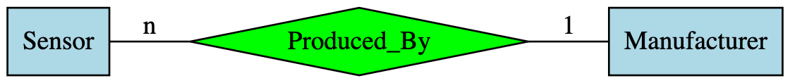
Note: Many-to-one and one-to-many are essentially the same relationship viewed from different directions. The arrow points toward the “one” side.
4. Many-to-Many (n:m or m:n)
Each entity in set A can be associated with multiple entities in set B, and each entity in B can be associated with multiple entities in A.
Example: Multiple Engineers can inspect a given Bridge, and each Engineer can inspect multiple Bridges.
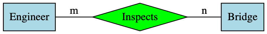
Notation: No arrows, or labels “n” and “m” (or “n” on both sides) indicating multiple on each side.
Relationship Attributes
Relationships themselves can have attributes! These are properties that belong to the connection between entities, not to the entities themselves.
Example: Consider the Inspects relationship between Engineer and Bridge. We might want to record:
Inspection_Date: When the inspection occurredCondition_Rating: The condition score assigned during that inspectionNotes: Comments from that specific inspection
These attributes don’t belong to the Engineer alone (one engineer performs many inspections on different dates), nor to the Bridge alone (a bridge is inspected multiple times). They belong to the relationship—the specific event of this engineer inspecting this bridge.
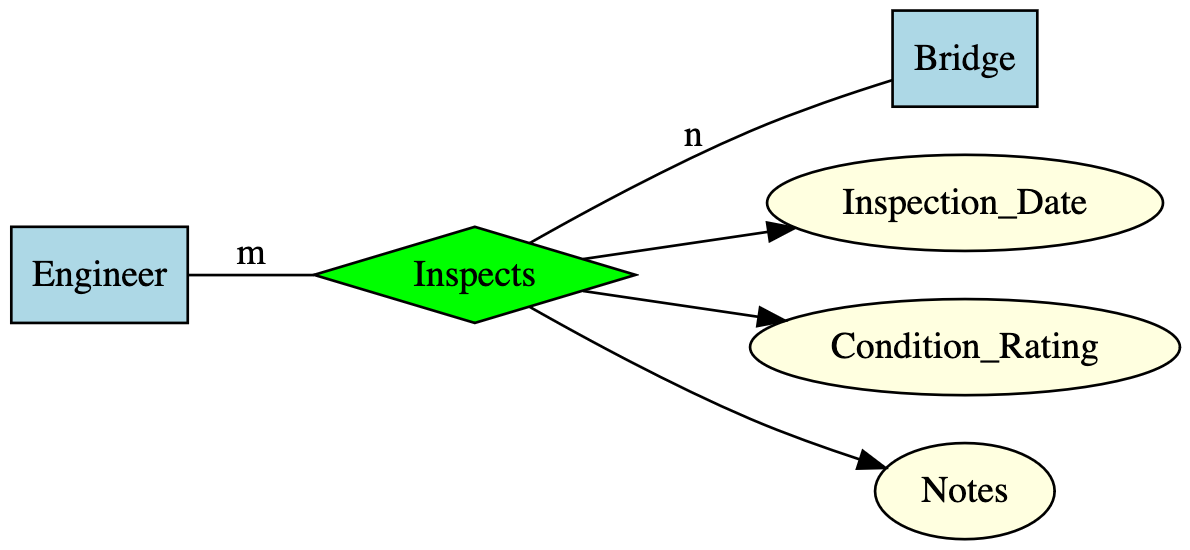
Key insight: Relationship attributes are especially common in many-to-many relationships, where they capture information about each specific connection between entities.
5.2.2.4 Weak Entity Sets
Sometimes, an entity set cannot uniquely identify its entities using only its own attributes. Instead, the identity of each entity depends partly on attributes from another related entity set. This leads to the concept of weak entity sets.
Definition: A weak entity set is an entity set whose key (unique identifier) is composed of attributes, some or all of which belong to another entity set. The weak entity set depends on another entity set (called its identifying or owner entity set) for its existence and identification.
Motivation and Common Scenarios:
The principal source of weak entity sets occurs when entity sets fall into a hierarchy of containment or ownership. If entity set E contains subunits that belong to entities in set F, the names or identifiers of E entities may not be unique across the entire system—they’re only unique within the context of their parent F entity.
Example 1: Rooms in Buildings
Consider a university campus database with Building and Room entity sets.
- Each building has a unique
Building_ID - Rooms are identified by
Room_Numberwithin a building - But
Room_Numberalone isn’t globally unique—many buildings have a “Room 101” - A room’s complete identity requires both its room number and the building it’s in
In this case, Room is a weak entity set:
- It depends on
Building(the identifying entity set) - Its key is a combination of its own
Room_Numberand theBuilding_IDfrom the related Building entity
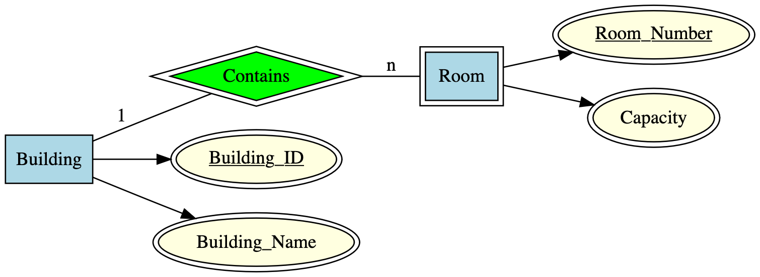
Notation:
- Weak entity sets are shown as rectangles with double borders (double-lined box)
- The identifying relationship (the many-one relationship connecting the weak entity to its owner) is shown as a diamond with double borders
- The partial key attribute (e.g.,
Room_Number) is underlined in the weak entity
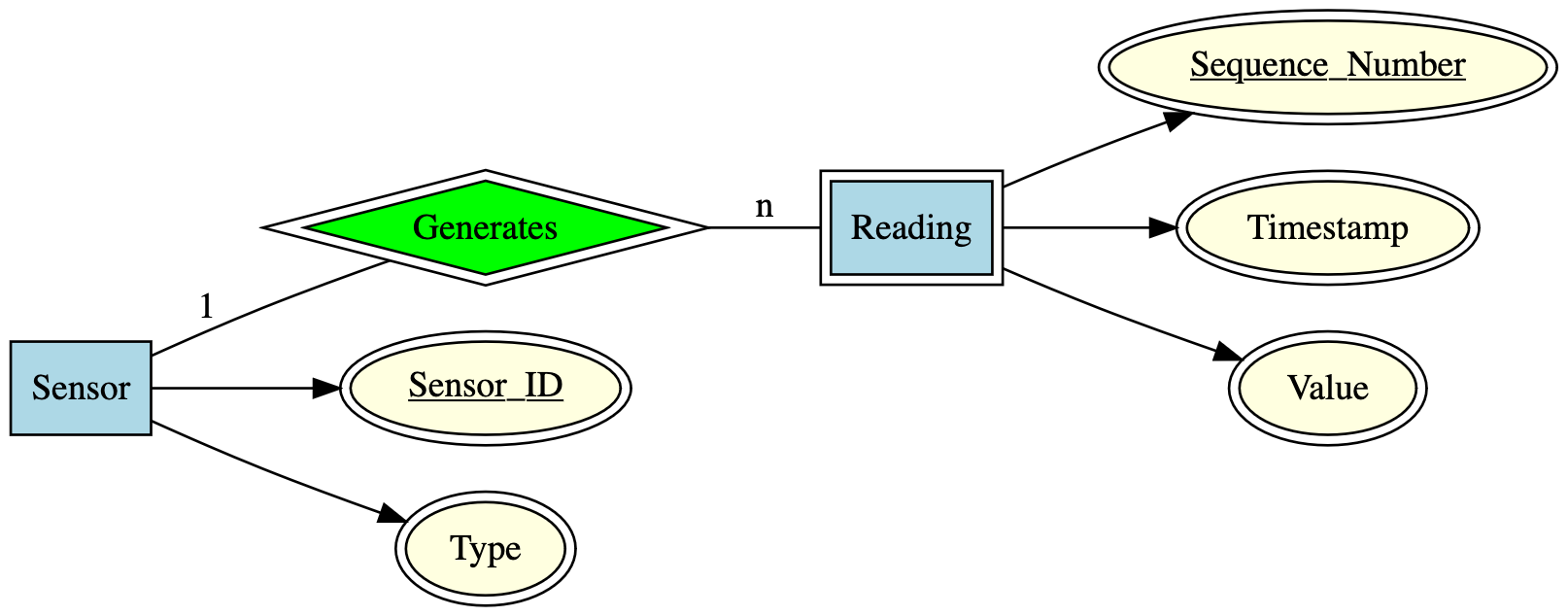
Example 2: Sensor Readings in a Monitoring System
Consider our bridge monitoring system. Suppose each sensor generates readings with sequential reading numbers:
Sensoris a regular (strong) entity with uniqueSensor_IDReadingentities are identified by aSequence_Number(1, 2, 3, …) within each sensor- But
Sequence_Numberalone doesn’t uniquely identify a reading globally—Sensor A’s reading #5 is different from Sensor B’s reading #5 - Each reading’s complete identity requires the
Sensor_IDplus its ownSequence_Number
Therefore, Reading is a weak entity set depending on Sensor:
Why distinguish weak entity sets?
- Conceptual clarity: Makes explicit the dependency between entities
- Database design: Affects how you create tables and foreign keys
- Integrity constraints: Weak entities cannot exist without their owner (if you delete a Building, all its Rooms must be deleted too—this is called a cascading delete)
- Key structure: Documents that the complete key is composite (spans multiple entity sets)
Key characteristics of weak entity sets:
- They have a partial key (discriminator)—an attribute that is unique only within the context of the owner entity
- They participate in an identifying relationship with their owner entity set
- The relationship is always many-to-one from the weak entity to the owner
- Weak entities cannot exist independently—they’re existentially dependent on their owner
5.2.2.5 Roles in Relationships
Sometimes, the same entity set participates in a relationship multiple times, playing different roles in each participation. When this happens, we need to explicitly label the roles to distinguish them.
When are roles needed?
Roles are necessary when:
- The same entity set appears two or more times in a single relationship
- We need to clarify which “side” of the relationship each participation represents
- The meaning of the relationship depends on distinguishing the different ways the entity participates
Example 1: Road Network
Consider a transportation database modeling road segments connecting intersections.
- Both endpoints of a road segment are intersections
- So the
Intersectionentity set appears twice in theConnectsrelationship - We need to distinguish the “start” intersection from the “end” intersection
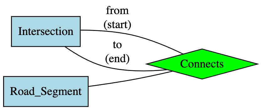
Here, the labels “from” and “to” are roles that clarify which intersection is the start point and which is the end point of the road segment.
Notation: We label the edges (lines) between the entity set and the relationship diamond with the role names.
Key insight: Roles are essential for clarity when an entity set relates to itself. Without role labels, it would be ambiguous which entity plays which part in the relationship.
5.2.2.6 Subclasses and ISA Hierarchies
Often, an entity set contains certain entities that have special properties not shared by all members of the set. Some entities are more specialized versions of the general entity type, with additional attributes or relationships.
Motivation: In these cases, it’s useful to define subclasses (also called subtypes or specializations)—special-case entity sets that inherit properties from a parent entity set but add their own specific attributes and relationships.
Definition: An ISA hierarchy (read as “is-a”) models inheritance where a subclass entity “is a” specialized version of the parent entity.
Example 1: Types of Bridges
Consider our bridge monitoring system. All bridges share common properties (location, year built, material), but different bridge types have type-specific attributes:
- Suspension bridges have cable properties (cable diameter, tower height, anchorage type)
- Truss bridges have truss configuration details (truss type, number of panels)
- Arch bridges have arch span and rise characteristics
Rather than adding all these specialized attributes to every bridge (leaving most empty), we create subclasses:
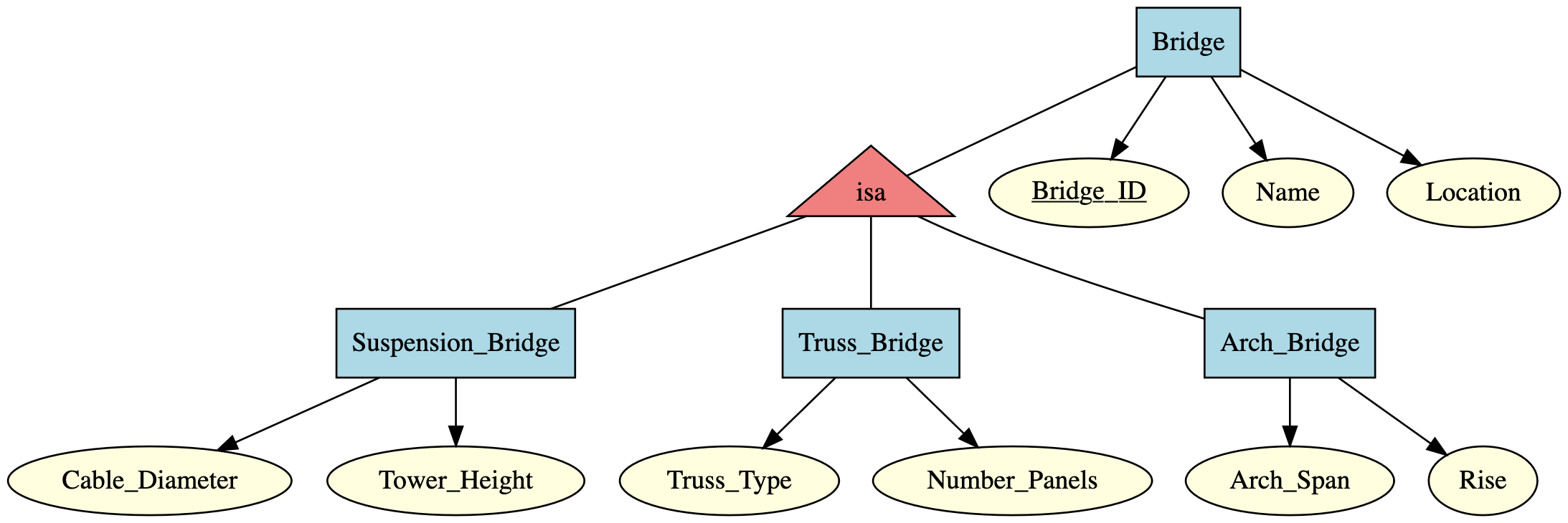
Reading this diagram:
Suspension_Bridge,Truss_Bridge, andArch_Bridgeare subclasses ofBridge- The triangle labeled “isa” represents the inheritance relationship
- Each suspension bridge is a bridge, so it has all Bridge attributes (ID, Name, Location) plus its specific attributes (Cable_Diameter, Tower_Height)
- Similarly for truss and arch bridges
Notation:
- Subclasses are connected to their parent (superclass) through a triangle labeled “isa”
- The triangle points toward the subclasses
- All ISA relationships are one-to-one (each subclass entity corresponds to exactly one parent entity)
- We don’t draw arrows on ISA relationships because the one-to-one nature is implicit
Properties of ISA Hierarchies:
- Inheritance: Subclasses inherit all attributes and relationships from their parent
- Specialization: Subclasses add their own specific attributes and relationships
- Substitutability: Anywhere a parent entity can appear, a subclass entity can appear (but not vice versa)
- Mutual exclusivity (often): An entity typically belongs to only one subclass (a bridge is either suspension or truss, not both)—though this isn’t always required
Why use subclasses?
- Clarity: Makes explicit which attributes apply to which entity types
- Efficiency: Avoids storing null values for attributes that don’t apply
- Extensibility: Easy to add new specialized types without modifying the parent
- Type-specific relationships: Subclasses can participate in relationships unique to their type
Real-world analogy: Think of biological taxonomy. A “Mammal” is a subclass of “Animal”—it inherits all animal properties (eats, moves, reproduces) but adds mammal-specific features (warm-blooded, has fur, nurses young). Similarly, “Dog” is a subclass of “Mammal,” further specializing the type.
5.2.2.7 Putting It All Together: A Complete ER Diagram
Now let’s integrate all the concepts we’ve learned into a comprehensive ER diagram for a realistic infrastructure monitoring system. This example will demonstrate entity sets, attributes (including key, multi-valued, and derived), relationships with different multiplicities, weak entity sets, roles, and subclasses.
Scenario: A city operates a structural health monitoring system for bridges. The system tracks:
- Bridges of different types (suspension, arch, truss)
- Sensors installed on bridges
- Engineers who maintain and inspect bridges
- Inspection events with condition ratings
- Sensor readings over time
Here’s the complete ER diagram:
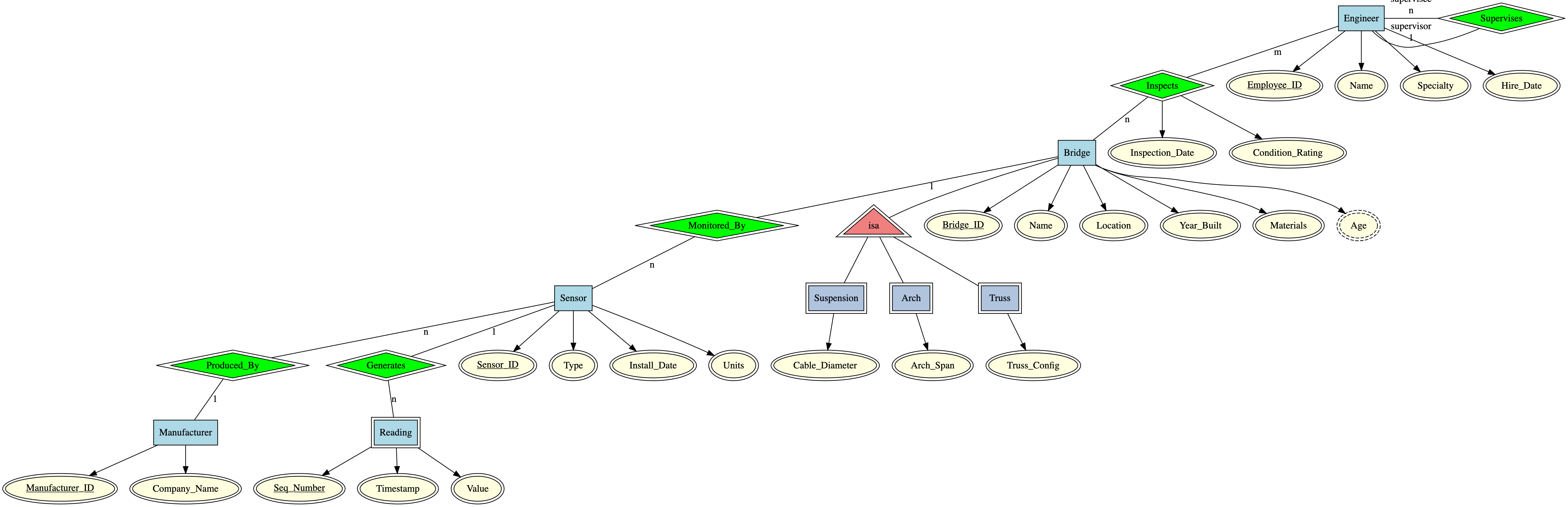
Reading this comprehensive diagram:
Entity Sets and Attributes:
- Bridge: Has
Bridge_ID(key),Name,Location,Year_Built,Materials(multi-valued - bridges can use multiple materials), andAge(derived fromYear_Built) - Engineer: Has
Employee_ID(key),Name,Specialty,Hire_Date - Sensor: Has
Sensor_ID(key),Type,Install_Date,Units - Manufacturer: Has
Manufacturer_ID(key),Company_Name - Reading (weak entity): Has
Seq_Number(partial key),Timestamp,Value
Relationships:
- Inspects (many-to-many): Engineers inspect bridges, with attributes
Inspection_DateandCondition_Ratingdescribing each inspection event - Monitored_By (one-to-many): Each bridge is monitored by many sensors
- Produced_By (many-to-one): Many sensors are produced by one manufacturer
- Generates (one-to-many, identifying): Each sensor generates many readings; Reading is a weak entity depending on Sensor
- Supervises (self-relationship with roles): Engineers supervise other engineers, with roles “supervisor” and “supervisee”
Subclasses (ISA Hierarchy):
- Suspension, Arch, and Truss are specialized types of bridges
- Each has type-specific attributes (cable diameter, arch span, truss configuration)
- They inherit all Bridge attributes
This diagram captures the complete structure of the monitoring system in a single visual representation. From this ER diagram, a database designer could:
- Identify all the tables needed
- Determine primary and foreign keys
- Understand entity dependencies and referential integrity constraints
- Plan for specialized storage of subclass-specific data
Design insights from this diagram:
- Readings are weak entities because they only make sense in the context of a specific sensor
- Materials is multi-valued because bridges often use multiple construction materials
- Age is derived to avoid redundant storage (can compute from
Year_Built) - Inspection attributes belong to the relationship, not to engineers or bridges alone
- The supervision hierarchy uses roles to clarify the asymmetric relationship among engineers
- Bridge subclasses allow type-specific attributes without cluttering the base Bridge entity
5.2.3 Set Theory for Data Management
5.2.3.1 Why Set Theory Matters for Databases
We’ve just learned how ER diagrams help us design the structure of a database—they tell us what entities and relationships we need. But once we’ve implemented a database, how do we actually work with the data?
This is where set theory becomes essential. Set theory provides the mathematical foundation for:
Understanding what data is: Every table in a database is fundamentally a set of records (rows). The entity set “Bridge” in our ER diagram becomes a set of bridge records in the database.
Querying data: When you ask a database “find all bridges built after 2000,” you’re asking for a subset of the bridge records. When you ask “find sensors that are on bridges AND manufactured by Company X,” you’re computing an intersection of two sets.
Combining data: Database operations like JOIN combine data from multiple tables using set operations. Understanding set theory helps you understand what these operations actually do.
Reasoning about data: Set theory gives us precise language to describe collections of data and relationships between collections.
The connection: Think of it this way:
- ER diagrams describe the structure (the blueprint)
- Set theory describes the data itself and operations on it (the mathematical foundation)
- Databases are the implementation (the actual system)
As we’ll see, operations you perform on database records—filtering, combining, selecting—are fundamentally set operations. Understanding set theory helps you think clearly about what your queries do and how to construct them correctly.
5.2.3.2 Sets: The Basics
5.2.3.2.1 Defining Sets
A set is a collection of distinct objects, considered as a single entity. The objects in a set are called elements or members of the set.
Key properties of sets:
- Unordered: The order of elements doesn’t matter. {A, B, C} is the same set as {C, A, B}
- Distinct: Each element appears only once. There’s no such thing as “two copies” of the same element in a set
- Well-defined: It must be clear whether any given object is in the set or not
Notation:
- Curly braces denote sets: \(S = \{a, b, c\}\)
- Capital letters typically denote sets: \(A, B, S, T\)
- Lowercase letters typically denote elements: \(a, b, x, y\)
- Membership: \(x \in S\) means “x is an element of S” (x is in S)
- Non-membership: \(x \notin S\) means “x is not an element of S”
Examples from engineering data:
Example 1: The set of bridges in our monitoring system: \[B = \{\text{Roberto Clemente Bridge, Fort Pitt Bridge, Fort Duquesne Bridge}\}\]
Example 2: The set of sensor types: \[T = \{\text{accelerometer, strain\_gauge, temperature, displacement}\}\]
Example 3: The set of inspection years for a particular bridge: \[Y = \{2018, 2019, 2020, 2021, 2022, 2023, 2024\}\]
Set-builder notation:
Often, we define sets by specifying a property that elements must satisfy, rather than listing all elements. This is called set-builder notation:
\[S = \{x \mid \text{condition on } x\}\]
Read as: “S is the set of all x such that x satisfies this condition”
Engineering examples:
- All bridges built after 2000: \(B_{new} = \{b \mid b \in Bridges \text{ and } b.year\_built > 2000\}\)
- All sensors with readings exceeding a threshold: \(S_{high} = \{s \mid s \in Sensors \text{ and } s.max\_reading > 100\}\)
- All engineers with civil specialization: \(E_{civil} = \{e \mid e \in Engineers \text{ and } e.specialty = \text{"Civil"}\}\)
Special sets:
- Empty set (denoted \(\emptyset\) or \(\{\}\)): The set with no elements. For example, if no bridges were built in 1950, then \(\{b \mid b.year\_built = 1950\} = \emptyset\)
- Universal set (denoted \(U\) or \(\Omega\)): The set of all elements under consideration in a given context. For our bridge database, the universal set might be all infrastructure assets in the city.
5.2.3.2.2 Subsets and Supersets
Sets can be related to each other through containment.
Definition: Set \(A\) is a subset of set \(B\) (written \(A \subseteq B\)) if every element of \(A\) is also an element of \(B\).
Mathematically: \(A \subseteq B\) if and only if \(\forall x: (x \in A \Rightarrow x \in B)\)
(Read as: “for all x, if x is in A, then x is in B”)
Definition: Set \(B\) is a superset of set \(A\) (written \(B \supseteq A\)) if \(A \subseteq B\). In other words, B contains all elements of A (and possibly more).
Proper subsets: \(A\) is a proper subset of \(B\) (written \(A \subset B\) or \(A \subsetneq B\)) if \(A \subseteq B\) and \(A \neq B\) (meaning B has at least one element not in A).
Engineering examples:
Example 1: Let \(S\) be all sensors, and \(S_{temp}\) be all temperature sensors. Then: \[S_{temp} \subset S\]
Temperature sensors are a proper subset of all sensors.
Example 2: Let \(B\) be all bridges, and \(B_{2020}\) be bridges inspected in 2020: \[B_{2020} \subseteq B\]
The bridges inspected in 2020 form a subset of all bridges.
Example 3: Consider these sets: - \(E\) = all engineers in the database - \(E_{civil}\) = engineers with civil engineering specialty - \(E_{senior}\) = engineers with more than 10 years experience - \(E_{lead}\) = senior civil engineers
Then: \(E_{lead} \subseteq E_{senior}\), \(E_{lead} \subseteq E_{civil}\), and both \(E_{senior} \subseteq E\) and \(E_{civil} \subseteq E\)
Important properties:
- Every set is a subset of itself: \(A \subseteq A\)
- The empty set is a subset of every set: \(\emptyset \subseteq A\) for any set \(A\)
- Subset relation is transitive: if \(A \subseteq B\) and \(B \subseteq C\), then \(A \subseteq C\)
5.2.3.2.3 Set Membership and Cardinality
Set Membership:
We’ve already seen the membership notation:
- \(x \in A\): “x is an element of A” or “x belongs to A”
- \(x \notin A\): “x is not an element of A”
Example: If \(B = \{\text{Bridge A, Bridge B, Bridge C}\}\), then:
- \(\text{Bridge A} \in B\) (Bridge A is in the set)
- \(\text{Bridge D} \notin B\) (Bridge D is not in the set)
Important distinction: Be careful not to confuse membership (\(\in\)) with the subset relation (\(\subseteq\)):
- \(\text{Bridge A} \in B\) (an individual bridge is an element of the bridge set)
- \(\{\text{Bridge A}\} \subseteq B\) (a set containing one bridge is a subset of the bridge set)
Cardinality:
The cardinality of a set is the number of elements it contains. We denote it as \(|A|\) or \(\#A\) or sometimes \(card(A)\).
Examples:
- If \(B = \{\text{Bridge A, Bridge B, Bridge C}\}\), then \(|B| = 3\)
- If \(T = \{\text{accelerometer, strain\_gauge, temperature, displacement}\}\), then \(|T| = 4\)
- The empty set has cardinality zero: \(|\emptyset| = 0\)
Engineering application: Cardinality is useful for counting:
- How many sensors are installed? \(|Sensors|\)
- How many bridges were inspected in 2024? \(|\{b \mid b.last\_inspection = 2024\}|\)
- How many readings has a sensor generated? \(|\{r \mid r.sensor\_id = \text{"S001"}\}|\)
Properties:
- Cardinality is always non-negative: \(|A| \geq 0\)
- If \(A \subseteq B\), then \(|A| \leq |B|\) (subsets can’t be larger than their supersets)
- If \(A \subset B\) (proper subset), then \(|A| < |B|\)
5.2.3.3 Operations on Sets
Just as we can perform arithmetic operations on numbers (addition, multiplication), we can perform operations on sets to create new sets. These operations are fundamental to database queries and data manipulation.
5.2.3.3.1 Union
The union of two sets contains all elements that are in either set (or both).
Definition: The union of sets \(A\) and \(B\), denoted \(A \cup B\), is: \[A \cup B = \{x \mid x \in A \text{ or } x \in B\}\]
Read as: “A union B is the set of all x such that x is in A or x is in B (or both)”
Key point: The “or” here is inclusive—an element is in the union if it’s in A, or in B, or in both.
Example 1: Simple sets
Let \(A = \{1, 2, 3\}\) and \(B = \{3, 4, 5\}\). Then: \[A \cup B = \{1, 2, 3, 4, 5\}\]
Note that 3 appears in both sets, but it only appears once in the union (sets contain distinct elements).
Example 2: Engineering application
Let \(B_{steel}\) be the set of steel bridges and \(B_{concrete}\) be the set of concrete bridges:
\[B_{steel} \cup B_{concrete} = \{\text{all bridges made of steel or concrete}\}\]
This represents all bridges built from either material.
Example 3: Sensor data
Let \(S_{2023}\) be sensors installed in 2023 and \(S_{2024}\) be sensors installed in 2024:
\[S_{2023} \cup S_{2024} = \{\text{all sensors installed in 2023 or 2024}\}\]
Properties of union:
- Commutative: \(A \cup B = B \cup A\) (order doesn’t matter)
- Associative: \((A \cup B) \cup C = A \cup (B \cup C)\)
- Identity element: \(A \cup \emptyset = A\) (union with empty set does nothing)
- Idempotent: \(A \cup A = A\) (unioning a set with itself gives the same set)
5.2.3.3.2 Intersection
The intersection of two sets contains only elements that are in both sets.
Definition: The intersection of sets \(A\) and \(B\), denoted \(A \cap B\), is: \[A \cap B = \{x \mid x \in A \text{ and } x \in B\}\]
Read as: “A intersection B is the set of all x such that x is in both A and B”
Example 1: Simple sets
Let \(A = \{1, 2, 3, 4\}\) and \(B = \{3, 4, 5, 6\}\). Then: \[A \cap B = \{3, 4\}\]
Only elements in both sets appear in the intersection.
Example 2: Engineering application
Let \(B_{old}\) be bridges built before 1950 and \(B_{steel}\) be steel bridges:
\[B_{old} \cap B_{steel} = \{\text{bridges that are both old AND made of steel}\}\]
This represents old steel bridges.
Example 3: Database query
Let \(E_{civil}\) be engineers with civil specialty and \(E_{senior}\) be engineers with >10 years experience:
\[E_{civil} \cap E_{senior} = \{\text{senior civil engineers}\}\]
This is exactly how database queries with multiple conditions work—you’re finding the intersection of multiple constraint sets.
Properties of intersection:
- Commutative: \(A \cap B = B \cap A\)
- Associative: \((A \cap B) \cap C = A \cap (B \cap C)\)
- Identity element: \(A \cap U = A\) where \(U\) is the universal set
- Zero element: \(A \cap \emptyset = \emptyset\) (intersection with empty set is always empty)
- Idempotent: \(A \cap A = A\)
5.2.3.3.3 Set Difference
The set difference (or relative complement) contains elements that are in the first set but not in the second set.
Definition: The set difference of \(A\) and \(B\), denoted \(A \setminus B\) or \(A - B\), is: \[A \setminus B = \{x \mid x \in A \text{ and } x \notin B\}\]
Read as: “A minus B is the set of all x such that x is in A but not in B”
Important: Set difference is not commutative—\(A \setminus B\) is generally different from \(B \setminus A\).
Example 1: Simple sets
Let \(A = \{1, 2, 3, 4\}\) and \(B = \{3, 4, 5, 6\}\). Then: \[A \setminus B = \{1, 2\}\] \[B \setminus A = \{5, 6\}\]
Example 2: Engineering application
Let \(B\) be all bridges and \(B_{inspected}\) be bridges inspected this year:
\[B \setminus B_{inspected} = \{\text{bridges NOT yet inspected this year}\}\]
This gives you the bridges that still need inspection—a practical query!
Example 3: Sensor maintenance
Let \(S\) be all sensors and \(S_{faulty}\) be sensors reporting errors:
\[S \setminus S_{faulty} = \{\text{sensors that are working correctly}\}\]
Properties of set difference:
- Not commutative: \(A \setminus B \neq B \setminus A\) (in general)
- \(A \setminus \emptyset = A\) (removing nothing changes nothing)
- \(A \setminus A = \emptyset\) (removing all elements leaves the empty set)
- \(A \setminus B = \emptyset\) if and only if \(A \subseteq B\)
5.2.3.3.4 Complement
The complement of a set contains all elements in the universal set that are not in the given set.
Definition: The complement of set \(A\), denoted \(A^c\) or \(\overline{A}\) or \(A'\), is: \[A^c = \{x \mid x \in U \text{ and } x \notin A\}\]
where \(U\) is the universal set (the set of all elements under consideration).
Equivalently: \(A^c = U \setminus A\)
Important: The complement depends on what you define as your universal set.
Example 1: Simple example
Let \(U = \{1, 2, 3, 4, 5, 6, 7, 8, 9, 10\}\) and \(A = \{2, 4, 6, 8, 10\}\) (even numbers). Then: \[A^c = \{1, 3, 5, 7, 9\}\] (odd numbers)
Example 2: Engineering application
Let \(U\) be all bridges in the city and \(B_{old}\) be bridges built before 1950:
\[B_{old}^c = \{\text{bridges built in 1950 or later}\}\]
Example 3: Database application
Let \(U\) be all sensors and \(S_{active}\) be sensors currently transmitting data:
\[S_{active}^c = \{\text{sensors that are inactive or offline}\}\]
Properties of complement:
- Double complement: \((A^c)^c = A\) (complement of complement gives back the original)
- Complement of universal set: \(U^c = \emptyset\)
- Complement of empty set: \(\emptyset^c = U\)
- De Morgan’s Laws (very important):
- \((A \cup B)^c = A^c \cap B^c\)
- \((A \cap B)^c = A^c \cup B^c\)
De Morgan’s Laws in plain language:
- “NOT (A or B)” is the same as “(NOT A) and (NOT B)”
- “NOT (A and B)” is the same as “(NOT A) or (NOT B)”
These are fundamental to logic and database queries!
5.2.3.3.5 Cartesian Product
The Cartesian product creates a set of ordered pairs by combining elements from two sets. This operation is fundamental to understanding how database tables relate to each other.
Definition: The Cartesian product of sets \(A\) and \(B\), denoted \(A \times B\), is: \[A \times B = \{(a, b) \mid a \in A \text{ and } b \in B\}\]
Read as: “A cross B is the set of all ordered pairs (a,b) where a is in A and b is in B”
Important: The result is a set of ordered pairs—(a,b) is different from (b,a).
Example 1: Simple sets
Let \(A = \{1, 2\}\) and \(B = \{x, y\}\). Then: \[A \times B = \{(1,x), (1,y), (2,x), (2,y)\}\]
Notice: \(|A \times B| = |A| \times |B| = 2 \times 2 = 4\)
Example 2: Engineers and Bridges
Let \(E = \{\text{Alice, Bob}\}\) (engineers) and \(B = \{\text{Bridge A, Bridge B}\}\) (bridges). Then: \[E \times B = \{(\text{Alice, Bridge A}), (\text{Alice, Bridge B}), (\text{Bob, Bridge A}), (\text{Bob, Bridge B})\}\]
This represents all possible pairings of engineers with bridges—exactly what you get when you JOIN two database tables without any filtering condition!
Example 3: Sensor locations and types
Let \(L = \{\text{North, South, East, West}\}\) (locations) and \(T = \{\text{temperature, strain}\}\) (sensor types). Then: \[L \times T = \{(\text{North, temperature}), (\text{North, strain}), (\text{South, temperature}), \ldots\}\]
This gives all possible combinations of locations and sensor types—8 possibilities total.
Connection to Database Tables:
The Cartesian product is exactly what happens when you JOIN two tables without any conditions:
SELECT * FROM Engineers, Bridges;This query produces \(|Engineers| \times |Bridges|\) rows—every engineer paired with every bridge. That’s why we usually add WHERE conditions to filter the Cartesian product down to meaningful relationships!
Properties of Cartesian product:
- Not commutative: \(A \times B \neq B \times A\) (order matters in ordered pairs)
- Cardinality: \(|A \times B| = |A| \times |B|\)
- Associative (in a sense): \((A \times B) \times C \cong A \times (B \times C) \cong A \times B \times C\) (can extend to triples, etc.)
- \(A \times \emptyset = \emptyset\) (product with empty set is empty)
Extended Cartesian product:
We can extend to multiple sets: \(A_1 \times A_2 \times \cdots \times A_n\) produces n-tuples (ordered sequences of n elements).
Database connection: A database table with n columns can be viewed as a subset of a Cartesian product:
\[\text{Bridge table} \subseteq \text{IDs} \times \text{Names} \times \text{Locations} \times \text{Years} \times \ldots\]
Not all possible combinations appear—only valid, meaningful bridge records. But the structure is fundamentally a Cartesian product filtered by constraints.
5.2.3.4 Visualizing Sets with Venn Diagrams
Venn diagrams are visual representations of sets and their relationships using overlapping circles (or other closed curves). They provide an intuitive way to understand set operations and relationships.
Basic structure:
- Each set is represented by a circle or closed curve
- The universal set \(U\) is typically represented by a rectangle containing all circles
- Elements are points inside the circles
- Overlapping regions represent intersections
How to read Venn diagrams:
The position of a point tells you which set(s) it belongs to:
- Inside circle A only → element is in \(A \setminus B\)
- Inside circle B only → element is in \(B \setminus A\)
- In the overlap of A and B → element is in \(A \cap B\)
- Outside both circles (but in rectangle) → element is in \((A \cup B)^c\)
Example: Bridge classification
Consider bridges classified by two properties: material (steel vs. not steel) and age (old vs. new).
Let: - \(S\) = set of steel bridges - \(O\) = set of old bridges (built before 1950)
The Venn diagram divides all bridges into four regions:
- \(S \cap O\): Old steel bridges
- \(S \cap O^c\): New steel bridges
- \(S^c \cap O\): Old non-steel bridges
- \(S^c \cap O^c\): New non-steel bridges
Translating between notation and diagrams:
Practice moving back and forth between symbolic notation and visual representation:
| Set Expression | Description | Visual Region |
|---|---|---|
| \(A \cap B\) | Elements in both A and B | Overlap of circles |
| \(A \cup B\) | Elements in either A or B (or both) | Both circles combined |
| \(A \setminus B\) | Elements in A but not B | Part of A circle not overlapping B |
| \((A \cup B)^c\) | Elements in neither A nor B | Outside both circles |
| \(A^c \cap B^c\) | Elements in neither A nor B (same as above) | Outside both circles |
Complex expressions:
Venn diagrams help verify identities like De Morgan’s Laws:
- \((A \cup B)^c\) (complement of union) and \(A^c \cap B^c\) (intersection of complements) shade the same region
- \((A \cap B)^c\) (complement of intersection) and \(A^c \cup B^c\) (union of complements) shade the same region
Three-set Venn diagrams:
With three sets, you get more complex overlapping patterns—up to 8 distinct regions representing all possible combinations of membership:
- In none of the sets
- In only A, only B, or only C
- In A and B but not C, A and C but not B, or B and C but not A
- In all three sets: \(A \cap B \cap C\)
Engineering application:
Consider monitoring system alerts with three conditions:
- \(H\) = high strain readings
- \(V\) = high vibration readings
- \(T\) = temperature anomalies
Engineers might want to query different regions:
- \(H \cap V \cap T\): Bridges with all three alert types (critical priority)
- \(H \cup V \cup T\): Bridges with any alert type (all monitored bridges)
- \(H \cap V \cap T^c\): High strain and vibration but normal temperature
- \((H \cup V \cup T)^c\): Bridges with no alerts (all clear)
Venn diagrams make these queries visually intuitive.
5.2.3.5 Properties of Set Operations
Understanding the algebraic properties of set operations helps you manipulate set expressions, simplify queries, and reason about data.
5.2.3.5.1 Commutative Property
An operation is commutative if the order of operands doesn’t matter.
Commutative operations:
- Union: \(A \cup B = B \cup A\)
- Example: (Steel bridges) ∪ (Old bridges) = (Old bridges) ∪ (Steel bridges)
- Intersection: \(A \cap B = B \cap A\)
- Example: (Civil engineers) ∩ (Senior staff) = (Senior staff) ∩ (Civil engineers)
Non-commutative operations:
- Set difference: \(A \setminus B \neq B \setminus A\) (generally)
- Example: (All sensors) (Faulty sensors) ≠ (Faulty sensors) (All sensors)
- The first gives working sensors; the second is empty!
- Cartesian product: \(A \times B \neq B \times A\)
- Example: Engineers × Bridges ≠ Bridges × Engineers
- The ordered pairs \((e, b)\) and \((b, e)\) are different
5.2.3.5.2 Associative Property
An operation is associative if grouping doesn’t matter when combining three or more sets.
Associative operations:
- Union: \((A \cup B) \cup C = A \cup (B \cup C)\)
- You can write \(A \cup B \cup C\) without ambiguity
- Example: (Steel bridges) ∪ (Concrete bridges) ∪ (Wood bridges) groups any way
- Intersection: \((A \cap B) \cap C = A \cap (B \cap C)\)
- You can write \(A \cap B \cap C\) without ambiguity
- Example: Finding engineers who are civil AND senior AND experienced in bridges
Why this matters: Associativity means you can process multiple conditions in any order—useful for query optimization in databases.
5.2.3.5.3 Distributive Property
Distributive laws describe how one operation distributes over another.
Key distributive properties:
Intersection distributes over union: \[A \cap (B \cup C) = (A \cap B) \cup (A \cap C)\]
Example: Steel bridges that are (old or long) = (Steel bridges that are old) or (Steel bridges that are long)
Union distributes over intersection: \[A \cup (B \cap C) = (A \cup B) \cap (A \cup C)\]
Example: Sensors that are (temperature OR (strain AND high-precision)) = (temperature OR strain) AND (temperature OR high-precision)
Why this matters: These laws allow you to rewrite queries in equivalent forms, which can be more efficient to compute or clearer to understand.
Absorption laws (related):
- \(A \cup (A \cap B) = A\)
- \(A \cap (A \cup B) = A\)
These simplify redundant conditions.
5.2.3.5.4 Special Sets and Relationships
Empty Set (\(\emptyset\)):
Properties:
- \(A \cup \emptyset = A\) (union identity)
- \(A \cap \emptyset = \emptyset\) (intersection with empty is empty)
- \(A \setminus \emptyset = A\)
- \(\emptyset \subseteq A\) for all A (empty set is subset of everything)
Universal Set (\(U\)):
Properties:
- \(A \cup U = U\)
- \(A \cap U = A\) (intersection identity)
- \(A \subseteq U\) for all A in the context
- \(U^c = \emptyset\)
Complementary Sets:
Two sets \(A\) and \(B\) are complementary if:
- \(A \cup B = U\) (together they cover everything)
- \(A \cap B = \emptyset\) (they don’t overlap)
- \(B = A^c\) (B is the complement of A)
Example: Active sensors and inactive sensors are complementary—every sensor is either active or inactive, but not both.
Disjoint Sets:
Two sets \(A\) and \(B\) are disjoint (or mutually exclusive) if: \[A \cap B = \emptyset\]
They have no elements in common.
Examples:
- Suspension bridges and truss bridges are disjoint (a bridge can’t be both types)
- Sensors installed in 2020 and sensors installed in 2021 are disjoint
- Temperature sensors and strain gauges might be disjoint (if types don’t overlap)
Properties of disjoint sets:
- If \(A\) and \(B\) are disjoint: \(|A \cup B| = |A| + |B|\)
- This is the addition principle of counting
Partition:
A collection of sets \(A_1, A_2, \ldots, A_n\) is a partition of set \(S\) if:
- They’re mutually disjoint: \(A_i \cap A_j = \emptyset\) for \(i \neq j\)
- Their union is \(S\): \(A_1 \cup A_2 \cup \cdots \cup A_n = S\)
- None are empty: \(A_i \neq \emptyset\)
Example: Bridge types (suspension, truss, arch, beam) partition the set of all bridges—every bridge is exactly one type.
Why partitions matter: They’re fundamental to classification systems and database table designs. Entity subclasses in ER diagrams often represent partitions.
5.2.3.6 Connecting Sets to ER Diagrams
Now we can bring everything together: ER diagrams describe structure, set theory provides the mathematical foundation, and database queries perform set operations.
5.2.3.6.1 Entity Sets as Sets
Every entity set in an ER diagram corresponds to a set in set theory:
- The Bridge entity set → the set of all bridge records
- The Sensor entity set → the set of all sensor records
- Each entity (a specific bridge) → an element of the set
Attributes define subsets:
- Bridges built after 2000 → \(\{b \in Bridges \mid b.year\_built > 2000\}\) (a subset)
- Steel bridges → \(\{b \in Bridges \mid \text{"steel"} \in b.materials\}\) (a subset)
5.2.3.6.2 Relationships as Set Operations
One-to-many relationships can be expressed using sets:
For the relationship “Bridge is monitored by Sensors”:
- For each bridge \(b\), there’s a set of sensors: \(Sensors(b) = \{s \in Sensors \mid s.bridge\_id = b.id\}\)
- Finding all sensors on any bridge in set \(B_{subset}\): \[\bigcup_{b \in B_{subset}} Sensors(b)\]
Many-to-many relationships are subsets of Cartesian products:
The “Engineer Inspects Bridge” relationship is a subset of \(Engineers \times Bridges\): \[Inspects \subseteq Engineers \times Bridges\]
Not every \((engineer, bridge)\) pair is in the relationship—only those where that engineer actually inspected that bridge.
5.2.3.6.3 Queries as Set Operations
WHERE clause = intersection:
SELECT * FROM Bridges
WHERE material = 'steel' AND year_built > 2000;
This computes: \(B_{steel} \cap B_{new}\)
OR conditions = union:
SELECT * FROM Bridges
WHERE material = 'steel' OR material = 'concrete';
This computes: \(B_{steel} \cup B_{concrete}\)
NOT conditions = complement or difference:
SELECT * FROM Bridges
WHERE bridge_id NOT IN (SELECT bridge_id FROM Inspections WHERE year = 2024);
This computes: \(Bridges \setminus Bridges_{inspected\_2024}\)
JOIN = Cartesian product + filter:
SELECT * FROM Engineers JOIN Bridges ON Engineers.specialty = Bridges.type;This computes: \(\{(e, b) \in Engineers \times Bridges \mid e.specialty = b.type\}\)
(A filtered subset of the Cartesian product)
Aggregation = cardinality:
SELECT COUNT(*) FROM Sensors WHERE type = 'temperature';This computes: \(|S_{temperature}|\)
5.2.3.6.4 Design Implications
Understanding the set-theoretic foundation helps with:
- Query optimization: Recognizing equivalent set expressions
- \(A \cap (B \cup C) = (A \cap B) \cup (A \cap C)\) suggests different query plans
- Understanding results: Knowing what data you’ll get
- Cartesian product without JOIN condition explodes data size
- UNION removes duplicates (set union), UNION ALL doesn’t
- Constraint specification: Defining data integrity rules
- Disjoint subclasses → partition constraint
- Foreign keys → subset constraint (child IDs must be in parent IDs)
- Reasoning about coverage: Do your queries cover all cases?
- Have you partitioned the search space?
- Are conditions mutually exclusive or overlapping?
Example: Suppose you want to ensure all bridges are categorized by age. You might verify: \[(Bridges_{old} \cup Bridges_{new} = Bridges) \land (Bridges_{old} \cap Bridges_{new} = \emptyset)\]
This confirms old and new bridges form a partition—complete coverage, no overlap.