viewof qU = Inputs.range([0, 1000], {value: 500, step: 10, label: "True Upper Level (qU)"})
viewof qL = Inputs.range([0, 1000], {value: 300, step: 10, label: "True Lower Level (qL)"})
viewof sigmaU = Inputs.range([0, 200], {value: 150, step: 10, label: "Upper Sensor Noise (σU)"})
viewof sigmaL = Inputs.range([0, 200], {value: 150, step: 10, label: "Lower Sensor Noise (σL)"})
viewof h = Inputs.range([0.05, 0.5], {value: 0.1, step: 0.05, label: "Vertical Distance (h)"})4 Module 3: Processing Time Series Data
4.1 Module Overview
4.1.1 Learning Objectives
By the end of this module, students will be able to:
- Be able to calculate error propagation for linear Gaussian models
- Understand the reasons for why error propagation is different when models are not linear
- Be able to conduct outlier removal in time series using Chauvenet’s criterion
- Be able to follow the derivation of linear regression with linear and non-linear basis functions
- Use linear regression to interpolate or extrapolate from the time-series data that is available (estimating unobserved values in the time domain)
4.1.2 Topics Covered
- Error propagation for linear Gaussian models
- Non-linear models and error propagation
- Outlier removal using Chauvenet’s criterion
- Linear regression derivation (linear and non-linear basis functions)
- Time series interpolation and extrapolation
4.1.3 Project Milestones
Post on Piazza your specific group assignments and/or your need to join a group for the final project.
4.2 Source Material
4.2.1 Recap: Uncertainty of Measurements Under Noise
In Module 2, we introduced the concept that real-world sensors produce measurements corrupted by noise. Let’s revisit this fundamental idea and make it more concrete, as understanding measurement uncertainty is critical for everything we’ll do in processing time series data.
4.2.1.1 The Measurement Model
Imagine we want to measure the temperature in a room using a digital thermometer. The true temperature (which we’ll never know exactly) is some value \(q\). When we take a measurement with our sensor, we get a reading \(y\). If our sensor were perfect, we’d have \(y = q\). But real sensors aren’t perfect—they’re affected by electronic noise, environmental factors, and inherent measurement limitations.
We can model this imperfection mathematically as:
\[y = q + n\]
where:
- \(q\) is the true physical quantity we’re trying to measure
- \(y\) is our actual measurement (what the sensor reports)
- \(n\) is the measurement noise
For many practical sensors, this noise \(n\) can be well-approximated as additive white Gaussian noise. This means:
- The noise is additive (it simply adds to the true value)
- It’s white (noise at one time point doesn’t depend on noise at other time points)
- It follows a Gaussian (Normal) distribution with mean zero and some variance \(\sigma^2\)
We write this as: \(n \sim \mathcal{N}(0, \sigma^2)\)
4.2.1.2 Why Gaussian Noise?
You might wonder: why do we assume Gaussian noise? While not all noise is perfectly Gaussian, there are good reasons this assumption is both practical and theoretically justified:
- Central Limit Theorem: When noise comes from many small, independent sources (thermal noise, quantization errors, electromagnetic interference, etc.), their sum tends toward a Gaussian distribution
- Mathematical tractability: Gaussian distributions have nice mathematical properties that make analysis possible
- Empirical observation: Many real sensors do exhibit approximately Gaussian noise
4.2.1.3 Understanding Uncertainty
Now, what does this noise model tell us about uncertainty? There are two perspectives we might care about:
Forward uncertainty - \(P(y|q)\): “Given that the true value is \(q\), what measurement \(y\) might I observe?”
Since \(y = q + n\) and \(n \sim \mathcal{N}(0, \sigma^2)\), we have:
\[P(y|q) = \mathcal{N}(q, \sigma^2) \tag{4.1}\]
This says: if the true value is \(q\), our measurements will be normally distributed around \(q\) with variance \(\sigma^2\).
Inverse uncertainty - \(P(q|y)\): “Given that I observed measurement \(y\), what might the true value \(q\) be?”
This is actually what we care about most! There are many ways to arrive at this quantity. A simple one is to re-arrange our \(y = q + n\) equation. Since we were able to derive that \(P(y|q)\) is Normal in (Equation 4.1), we can easily see that \(q = y - n\) should also follow a distribution \(P(q|y)\) that is normal with mean \(y\) and variance \(\sigma^2\), namely:
\[P(q|y) = \mathcal{N}(y, \sigma^2)\]
This result shows that both distributions have the same form and the same variance. Given a measurement \(y\), our best estimate of the true value \(q\) is simply \(y\) itself, but we remain uncertain by an amount characterized by \(\sigma^2\).
4.2.1.4 Estimating the Noise Level
How do we determine \(\sigma^2\) in practice? If we can take multiple measurements \(y_1, y_2, \ldots, y_N\) of the same physical quantity \(q\) (which remains constant), we can estimate the variance from the sample variance:
\[\hat{\sigma}^2 = \frac{1}{N-1} \sum_{i=1}^{N} (y_i - \bar{y})^2\]
where \(\bar{y} = \frac{1}{N}\sum_{i=1}^{N} y_i\) is the sample mean.
This gives us a practical way to characterize our sensor’s uncertainty: collect repeated measurements under stable conditions and compute the sample variance.
4.2.2 Error Propagation for Virtual Sensors
In Module 2, we introduced the concept of virtual sensors—measurements that are computed from other sensor measurements rather than directly measured. For example, if we measure the water levels at the top and bottom of a dam, we might compute the pressure difference as a virtual sensor. A key question arises: if our physical sensors have uncertainty, how does that uncertainty propagate to our virtual sensors?
4.2.2.1 A Motivating Example: Averaging Two Measurements
Let’s start with the simplest possible case. Suppose we have two sensors measuring the same physical quantity \(q\):
\[y_1 = q + n_1, \quad n_1 \sim \mathcal{N}(0, \sigma_1^2)\] \[y_2 = q + n_2, \quad n_2 \sim \mathcal{N}(0, \sigma_2^2)\]
where \(n_1\) and \(n_2\) are independent (noise in one sensor doesn’t affect the other).
To get a better estimate, we might average the two measurements to create a virtual sensor:
\[z = \frac{1}{2}y_1 + \frac{1}{2}y_2\]
Question: What is the noise affecting \(z\)? Is it better or worse than using just one sensor?
Let’s work this out. Substituting our measurement model:
\[z = \frac{1}{2}(q + n_1) + \frac{1}{2}(q + n_2) = q + \frac{1}{2}n_1 + \frac{1}{2}n_2\]
So the virtual sensor has noise \(n_z = \frac{1}{2}n_1 + \frac{1}{2}n_2\). What are the properties of this noise?
Mean: Since both \(n_1\) and \(n_2\) have zero mean: \[E[n_z] = \frac{1}{2}E[n_1] + \frac{1}{2}E[n_2] = 0\]
Great! The virtual sensor is still unbiased (zero mean noise).
Variance: Using the independence of \(n_1\) and \(n_2\): \[\text{Var}(n_z) = \text{Var}\left(\frac{1}{2}n_1 + \frac{1}{2}n_2\right) = \frac{1}{4}\text{Var}(n_1) + \frac{1}{4}\text{Var}(n_2) = \frac{1}{4}\sigma_1^2 + \frac{1}{4}\sigma_2^2\]
Special case: If both sensors have the same noise level (\(\sigma_1 = \sigma_2 = \sigma\)), then: \[\text{Var}(n_z) = \frac{1}{4}\sigma^2 + \frac{1}{4}\sigma^2 = \frac{1}{2}\sigma^2\]
By averaging two independent measurements, we’ve reduced the variance by half. The standard deviation (the square root of variance) is reduced by a factor of \(\sqrt{2} \approx 0.707\). This is why taking multiple measurements and averaging them improves accuracy.
Distribution: Since \(n_1\) and \(n_2\) are Gaussian and we’re taking a linear combination, \(n_z\) is also Gaussian (this is a key property of Gaussian distributions). Therefore:
\[z = q + n_z, \quad n_z \sim \mathcal{N}\left(0, \frac{\sigma^2}{2}\right)\]
4.2.2.2 The General Linear Case
Now let’s generalize. Suppose we have \(m\) sensors measuring different (or the same) physical quantities:
\[y_k = q_k + n_k, \quad n_k \sim \mathcal{N}(0, \sigma_k^2), \quad k = 1, 2, \ldots, m\]
And we create a virtual sensor as a linear combination of these measurements:
\[z_i = \sum_{k=1}^{m} \alpha_k y_{k,i} + c\]
where \(\alpha_k\) are weighting coefficients and \(c\) is a constant offset.
Following the same logic as before:
\[z_i = \sum_{k=1}^{m} \alpha_k (q_k + n_k) + c = \left(\sum_{k=1}^{m} \alpha_k q_k + c\right) + \sum_{k=1}^{m} \alpha_k n_k\]
The virtual sensor has noise: \[n_z = \sum_{k=1}^{m} \alpha_k n_k\]
Mean: Still zero (since each \(n_k\) has zero mean)
Variance: Assuming independent noise across sensors: \[\text{Var}(n_z) = \sum_{k=1}^{m} \alpha_k^2 \sigma_k^2\]
Distribution: \(n_z \sim \mathcal{N}\left(0, \sum_{k=1}^{m} \alpha_k^2 \sigma_k^2\right)\)
Key insight: The variance of the virtual sensor depends on:
- The variances of the input sensors (\(\sigma_k^2\))
- The squares of the coefficients (\(\alpha_k^2\))
This means:
- Multiplying a measurement by a factor \(\alpha\) multiplies its variance by \(\alpha^2\)
- Adding independent noisy measurements adds their variances
- The constant \(c\) doesn’t affect uncertainty at all (it’s just a bias)
4.2.2.3 Interactive Exploration: Virtual Sensors in Action
Let’s make this concrete with an interactive example. Imagine we have two sensors measuring water levels at different locations in a reservoir system:
- Sensor 1 measures the upper level: \(y_{1,k} = q_U + n_{1,k}\)
- Sensor 2 measures the lower level: \(y_{2,k} = q_L + n_{2,k}\)
From these, we create two virtual sensors:
- Average level: \(z_A = \frac{1}{2}y_1 + \frac{1}{2}y_2\) (measures \(q_A = \frac{1}{2}q_U + \frac{1}{2}q_L\))
- Gradient (flow rate proxy): \(z_C = \frac{1}{h}y_1 - \frac{1}{h}y_2\) where \(h\) is the vertical distance between sensors
Use the interactive visualization below to explore how changing the true levels (\(q_U\), \(q_L\)) and noise levels (\(\sigma_U\), \(\sigma_L\)) affects both the raw measurements and the virtual sensors:
Note
The following activity needs to be completed in an interactive version of this document (i.e, the HTML output served by a webserver).
Experiment with the controls:
- Try increasing both \(\sigma_U\) and \(\sigma_L\)—watch how noise increases in all sensors
- Set \(q_U = q_L\)—the gradient should be near zero, but notice the noise!
- Decrease \(h\) (sensors closer together)—the gradient uncertainty explodes!
- Compare the scatter in the average plot versus the individual sensor plots
This interactive example illustrates a crucial engineering trade-off: virtual sensors that amplify measurements (large coefficients) also amplify noise.
4.2.2.4 When Things Go Non-Linear: Breaking the Gaussian Assumption
Everything we’ve discussed so far relies on a critical assumption: the virtual sensor is a linear function of the measurements. But what happens when the relationship is non-linear?
Consider a practical example: measuring power dissipation in a resistor. If we measure current \(I\) flowing through a resistor with resistance \(R\):
\[I_{measured} = I_{true} + n_I, \quad n_I \sim \mathcal{N}(0, \sigma_I^2)\]
The power dissipated is given by Joule’s law (a non-linear operation with a squared term):
\[P = I^2 R\]
This raises two critical questions: 1. If \(I\) follows a Gaussian distribution, does \(P\) also follow a Gaussian distribution? 2. If not, what does the distribution of our computed power actually look like?
Let’s explore both questions with a simulation:
Code
import numpy as np
import matplotlib.pyplot as plt

# Set random seed for reproducibility
np.random.seed(42)

# True values
I_true = 0.5    # amperes
R = 1        # ohms (known, no noise)
P_true = I_true**2 * R  # watts (true power dissipation)

# Noise level - relatively high to emphasize non-linear effects
sigma_I = 1   # amperes (200% relative noise)

# Generate many samples
N = 10000
I_measured = I_true + np.random.normal(0, sigma_I, N)

# Compute power using non-linear squared relationship
P_measured = I_measured**2 * R

# Compute errors
error_P = P_measured - P_true

# Create figure with two subplots
fig, axes = plt.subplots(1, 2, figsize=(14, 5))

# Left plot: Distribution of power measurements vs Gaussian
axes[0].hist(P_measured, bins=50, density=True, alpha=0.7, color='blue',
             edgecolor='black', label='Actual P distribution')

# Overlay what a Gaussian with the same mean and variance would look like
mean_P = np.mean(P_measured)
std_P = np.std(P_measured)
x_P = np.linspace(P_measured.min(), P_measured.max(), 100)
gaussian_P = (1/(std_P * np.sqrt(2*np.pi))) * np.exp(-0.5*((x_P - mean_P)/std_P)**2)
axes[0].plot(x_P, gaussian_P, 'r-', linewidth=2, label=f'Gaussian N({mean_P:.1f}, {std_P:.1f}²)')

axes[0].axvline(P_true, color='green', linestyle='--', linewidth=2, label=f'True Power = {P_true:.1f}W')
axes[0].set_xlabel('Measured Power (W)')
axes[0].set_ylabel('Probability Density')
axes[0].set_title('Power Distribution: I ~ Gaussian ≠> P ~ Gaussian\n(Non-linear: P = I²R)')
axes[0].legend()
axes[0].grid(True, alpha=0.3)

# Right plot: Distribution of errors with Gaussian overlay
axes[1].hist(error_P, bins=50, density=True, alpha=0.7, color='orange', edgecolor='black', label='Actual error distribution')

# Overlay what a Gaussian with the same mean and variance would look like
mean_error = np.mean(error_P)
std_error = np.std(error_P)
x = np.linspace(error_P.min(), error_P.max(), 100)
gaussian_overlay = (1/(std_error * np.sqrt(2*np.pi))) * np.exp(-0.5*((x-mean_error)/std_error)**2)
axes[1].plot(x, gaussian_overlay, 'r-', linewidth=2, label=f'Gaussian N({mean_error:.1f}, {std_error:.1f}²)')

axes[1].set_xlabel('Error in Power (W)')
axes[1].set_ylabel('Probability Density')
axes[1].set_title('Error Distribution vs Gaussian\n(Notice: NOT quite Gaussian!)')
axes[1].legend()
axes[1].grid(True, alpha=0.3)

plt.tight_layout()
plt.show()

# Print statistics
print(f"True Power: {P_true} W")
print(f"Mean Measured Power: {np.mean(P_measured):.2f} W")
print(f"Std Dev of Power: {np.std(P_measured):.2f} W")
print(f"\nError Statistics:")
print(f"  Mean error: {mean_error:.2f} W (should be ~0 for Gaussian)")
print(f"  Std dev: {std_error:.2f} W")
print(f"  Skewness: {np.mean(((error_P - mean_error)/std_error)**3):.3f} (0 for Gaussian)")
print(f"  Kurtosis: {np.mean(((error_P - mean_error)/std_error)**4):.3f} (3 for Gaussian)")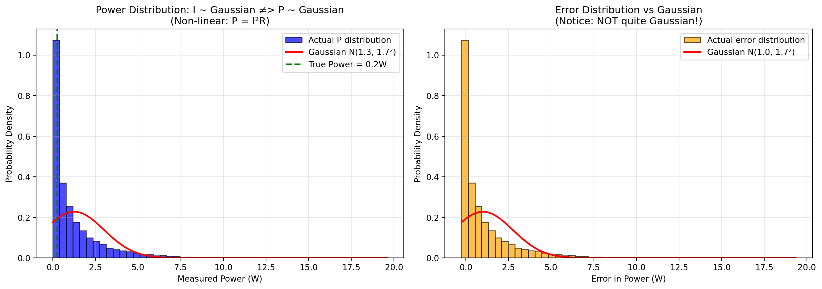
True Power: 0.25 W
Mean Measured Power: 1.25 W
Std Dev of Power: 1.75 W

Error Statistics:
  Mean error: 1.00 W (should be ~0 for Gaussian)
  Std dev: 1.75 W
  Skewness: 2.729 (0 for Gaussian)
  Kurtosis: 13.906 (3 for Gaussian)
Key Observations:
The power distribution itself is NOT Gaussian (left plot): Even though the current measurements \(I\) follow a Gaussian distribution, the computed power \(P = I^2 R\) does not. The actual distribution (blue histogram) is completely different to what a Gaussian with the same mean and variance would look like (red curve). This is a fundamental consequence: non-linear transformations of Gaussian variables are generally not Gaussian. The main driving force here is the fact that power measurements are never below zero, whereas the Gaussian distribution does allow for negative values.
The error distribution is also NOT Gaussian (right plot): Similarly, the error in power estimates shows pronounced positive skew (right tail). The distribution is visibly asymmetric, and the skewness statistic deviates significantly from zero. The kurtosis also differs notably from 3 (the value for a true Gaussian).
The mean error is positive (positive bias): Even though the input noise \(n_I\) has zero mean, the mean of the power error is positive! This is because of the squared term: \[(I_{true} + n_I)^2 R = I_{true}^2 R + 2I_{true}n_I R + n_I^2 R\] The last term \(n_I^2 R\) is always positive (since it’s squared), creating a positive bias in the power estimates. Specifically, \(E[n_I^2] = \sigma_I^2\), so the expected bias is \(R\sigma_I^2\).
The distribution is skewed right: Large positive noise values in \(I\) get amplified more than negative noise values because of the squaring.
Consequences for virtual sensors:
- We can’t assume the virtual sensor output is Gaussian just because inputs are Gaussian
- We can’t use simple linear error propagation formulas
- Confidence intervals based on Gaussian assumptions will be systematically wrong
- For non-linear transformations, Monte Carlo simulation (like above) or analytical approaches like the Delta method become necessary
- Simple averaging won’t give unbiased estimates of the true power
When is this a problem?: If the noise is small relative to the signal (high signal-to-noise ratio), the non-linearity matters less. But when noise is significant or the function is highly non-linear (e.g., squares, exponentials, divisions by small numbers), the Gaussian approximation breaks down completely.
4.2.3 Data Cleansing: Dealing with Messy Real-World Data
So far, we’ve assumed our sensor data follows nice theoretical models. Reality is messier. Real sensor data often suffers from:
- Incompleteness: Missing measurements due to communication failures, power outages, or sensor downtime
- Inconsistency: Contradictory readings from redundant sensors or physically impossible values
- Noise: Not just Gaussian noise, but also spikes, drift, and other artifacts
Data cleansing (also called data cleaning or preprocessing) is the process of detecting and correcting (or removing) these issues to prepare data for analysis.
4.2.3.1 The Two Faces of Outliers
An outlier is a measurement that deviates significantly from the expected pattern or trend. But here’s the critical question: what does it mean?
Sometimes outliers are the signal:
- A sudden spike in structural vibrations might indicate damage
- An unusual temperature reading might signal a fire
- Anomalous traffic patterns could indicate an accident
Sometimes outliers are noise:
- A communication error transmits garbage data
- A sensor briefly malfunctions
- Electromagnetic interference causes a spurious reading
The key is understanding your application: Are you looking for anomalies (keep the outliers!) or modeling normal behavior (remove them)?
4.2.3.2 Common Causes of Outliers
Physical perturbations: Real events that cause genuine deviations (e.g., a truck passing over a bridge causes a vibration spike)
Sensor malfunctioning: Hardware issues like degraded sensors, calibration drift, or component failure
Communication errors: Bit flips, packet loss, or transmission interference corrupting data in transit
Environmental factors: External conditions affecting sensor performance (temperature, humidity, electromagnetic fields)
4.2.3.3 Missing Values: Strategies for Handling Gaps
When data points are missing, you have several options:
| Strategy | When to Use | Pros | Cons |
|---|---|---|---|
| Ignore the gap | Time-series analysis methods that handle irregular sampling | Simple, no assumptions | Reduces effective sample size |
| Manual filling | Critical data with small gaps where you have context | Most accurate if done carefully | Not scalable, labor-intensive |
| Default/flag value | When you need complete arrays but want to mark missing data | Preserves data structure | Must remember to handle flags in analysis |
| Mean imputation | Random, occasional gaps in stationary signals | Simple, maintains mean | Reduces variance artificially |
| Linear interpolation | Smoothly varying signals with small gaps | Reasonable for smooth trends | Poor for rapidly changing signals |
Example: If you’re measuring bridge deflection (a smoothly varying quantity) and miss 2 readings in a sequence of 1000, linear interpolation is reasonable. But if you’re monitoring binary events (door open/closed), interpolation makes no physical sense.
4.2.3.4 Statistical Approach to Outlier Detection
A principled approach to outlier detection uses probabilistic reasoning:
Model the normal behavior: Estimate a probability distribution for typical measurements (e.g., Gaussian with mean \(\mu\) and variance \(\sigma^2\))
Compute probabilities: For each measurement, compute how likely it is under the model
Flag low-probability points: Measurements with very low probability are outliers
For Gaussian models, this translates to: “flag points that are too many standard deviations away from the mean.”
4.2.3.5 Quick Review: Sample Statistics
Before we dive into a specific outlier detection method, let’s recall how we estimate population parameters from samples.
If we have measurements \(y_1, y_2, \ldots, y_N\) from our model \(y_i = q + n_i\) where \(n_i \sim \mathcal{N}(0, \sigma^2)\):
Sample mean (estimates \(q\)): \[\bar{y} = \frac{1}{N} \sum_{i=1}^{N} y_i\]
Sample variance (estimates \(\sigma^2\)): \[s^2 = \frac{1}{N-1} \sum_{i=1}^{N} (y_i - \bar{y})^2\]
Sample standard deviation (estimates \(\sigma\)): \[s = \sqrt{s^2}\]
Note: We divide by \(N-1\) (not \(N\)) in the variance formula to get an unbiased estimate (Bessel’s correction).
These statistics will be the foundation of our outlier detection method.
4.2.3.6 Chauvenet’s Criterion: A Practical Outlier Detection Method
One of the most straightforward outlier detection methods is Chauvenet’s criterion, developed by the American astronomer William Chauvenet in the 1860s for cleaning astronomical observations.
4.2.3.6.1 The Basic Idea
The core principle is simple: Reject measurements that are “too far” from the mean, where “too far” is defined in terms of standard deviations.
But how far is “too far”? Chauvenet’s insight was to use probability: if the chance of observing a point that extreme (given the Gaussian model) is less than 1/(2N), where N is the sample size, then it’s likely an outlier rather than genuine variation.
4.2.3.6.2 Step-by-Step Procedure
Step 1: Compute the standardized distance
For each measurement \(y_i\), compute how many standard deviations it is from the mean:
\[d_i = \frac{|y_i - \bar{y}|}{s}\]
where \(\bar{y}\) is the sample mean and \(s\) is the sample standard deviation.
This is sometimes called the “z-score” or “standardized residual.”
Step 2: Choose a threshold
Common threshold choices based on the number of standard deviations:
| Threshold (\(d_{threshold}\)) | P(false rejection) | Typical Use |
|---|---|---|
| 1.0 | 31.7% | Too lenient (would reject valid data often) |
| 2.0 | 4.6% | Moderate (2-sigma rule) |
| 3.0 | 0.3% | Conservative (3-sigma rule) |
| 4.0 | 0.006% | Very conservative |
The probability shown is the chance that a genuinely Gaussian point would be this far from the mean by random chance (i.e., the probability of incorrectly rejecting a good measurement).
For Chauvenet’s original criterion, the threshold adapts to sample size N. A common rule: use \(d_{threshold}\) such that \(P(|Z| > d_{threshold}) < 1/(2N)\) where \(Z \sim \mathcal{N}(0,1)\).
Step 3: Reject or accept
- If \(d_i \leq d_{threshold}\): Accept the measurement
- If \(d_i > d_{threshold}\): Reject the measurement as an outlier
Step 4: Iterate
Here’s the crucial part: outliers contaminate our estimates of \(\bar{y}\) and \(s\)! If we have one extreme outlier, it pulls the mean toward it and inflates the standard deviation, making other outliers harder to detect.
Solution: Use an iterative approach:
- Compute \(\bar{y}\) and \(s\) from all data
- Apply Chauvenet’s criterion to identify outliers
- Remove identified outliers
- Recompute \(\bar{y}\) and \(s\) from remaining data
- Repeat steps 2-4 until no new outliers are found (convergence)
Typically, this converges in 2-4 iterations.
4.2.3.6.3 Example: Cleaning Temperature Data
Let’s apply Chauvenet’s criterion to a realistic example:
Note
In this example (and future ones) I am choosing to write out the simulation and experiments using Python. A good amount of the intuition about what we are trying to simulate in the example is encoded directly in the Python code (e.g., for this case, we are simulating 100 data points coming from a Normal distribution with mean 20 Celsius and standard deviation 0.5 degrees Celsius). As a result, you may need to read through the code in order to get a better understanding of the resulting plots.
Code
import numpy as np
import matplotlib.pyplot as plt
from scipy import stats

# Generate realistic temperature data with outliers
np.random.seed(123)
N = 100
true_temp = 20.0  # Celsius
noise_std = 0.5

# Generate mostly good data
temperatures = true_temp + np.random.normal(0, noise_std, N)

# Add some outliers (sensor glitches)
outlier_indices = [10, 25, 63, 87]
temperatures[outlier_indices] = [35.0, -5.0, 40.0, 32.0]

def chauvenets_criterion(data, threshold=2.0, max_iterations=10):
    """
    Apply Chauvenet's criterion iteratively to remove outliers.
    Returns: cleaned data, indices of outliers, iteration history
    """
    data = np.array(data, dtype=float)
    valid_mask = np.ones(len(data), dtype=bool)
    history = []

    for iteration in range(max_iterations):
        # Compute statistics on currently valid data
        valid_data = data[valid_mask]
        mean = np.mean(valid_data)
        std = np.std(valid_data, ddof=1)

        # Compute standardized distances for ALL points
        d = np.abs(data - mean) / std

        # Find outliers (only among currently valid points)
        newly_rejected = valid_mask & (d > threshold)

        # Store history
        history.append({
            'iteration': iteration + 1,
            'mean': mean,
            'std': std,
            'n_valid': np.sum(valid_mask),
            'n_rejected_this_round': np.sum(newly_rejected)
        })

        # Check for convergence
        if np.sum(newly_rejected) == 0:
            break

        # Update valid mask
        valid_mask = valid_mask & ~newly_rejected

    outlier_indices = np.where(~valid_mask)[0]
    return data[valid_mask], outlier_indices, history

# Apply Chauvenet's criterion
cleaned_data, outlier_idx, history = chauvenets_criterion(temperatures, threshold=3.0)

# Print iteration history
print("Chauvenet's Criterion - Iteration History (threshold = 3.0 σ):")
print("-" * 70)
for h in history:
    print(f"Iteration {h['iteration']}: mean={h['mean']:.3f}, std={h['std']:.3f}, "
          f"valid points={h['n_valid']}, rejected this round={h['n_rejected_this_round']}")
print("-" * 70)
print(f"Final result: {len(cleaned_data)} points retained, {len(outlier_idx)} outliers removed")
print(f"Detected outlier indices: {outlier_idx}")
print(f"Actual outlier indices:   {outlier_indices}")

# Visualization
fig, axes = plt.subplots(1, 2, figsize=(14, 5))

# Plot 1: Original data
axes[0].scatter(range(N), temperatures, c='blue', alpha=0.6, label='All data')
axes[0].scatter(outlier_indices, temperatures[outlier_indices],
                c='red', s=100, marker='x', linewidths=3, label='Known outliers')
axes[0].axhline(true_temp, color='green', linestyle='--', linewidth=2, label='True temperature')
axes[0].set_xlabel('Measurement index')
axes[0].set_ylabel('Temperature (°C)')
axes[0].set_title('Original Data with Outliers')
axes[0].legend()
axes[0].grid(True, alpha=0.3)

# Plot 2: After cleaning
valid_indices = np.arange(N)
valid_indices = np.delete(valid_indices, outlier_idx)
axes[1].scatter(valid_indices, cleaned_data, c='blue', alpha=0.6, label='Retained data')
axes[1].scatter(outlier_idx, temperatures[outlier_idx],
                c='red', s=100, marker='x', linewidths=3, label='Removed as outliers')
axes[1].axhline(true_temp, color='green', linestyle='--', linewidth=2, label='True temperature')
axes[1].set_xlabel('Measurement index')
axes[1].set_ylabel('Temperature (°C)')
axes[1].set_title('After Applying Chauvenet\'s Criterion')
axes[1].legend()
axes[1].grid(True, alpha=0.3)

plt.tight_layout()
plt.show()

# Compare statistics
print(f"\nStatistical comparison:")
print(f"Original data: mean={np.mean(temperatures):.3f}, std={np.std(temperatures, ddof=1):.3f}")
print(f"Cleaned data:  mean={np.mean(cleaned_data):.3f}, std={np.std(cleaned_data, ddof=1):.3f}")
print(f"True values:   mean={true_temp:.3f}, std={noise_std:.3f}")
Chauvenet's Criterion - Iteration History (threshold = 3.0 σ):
----------------------------------------------------------------------
Iteration 1: mean=20.253, std=3.785, valid points=100, rejected this round=4
Iteration 2: mean=20.034, std=0.569, valid points=96, rejected this round=0
----------------------------------------------------------------------
Final result: 96 points retained, 4 outliers removed
Detected outlier indices: [10 25 63 87]
Actual outlier indices: [10, 25, 63, 87]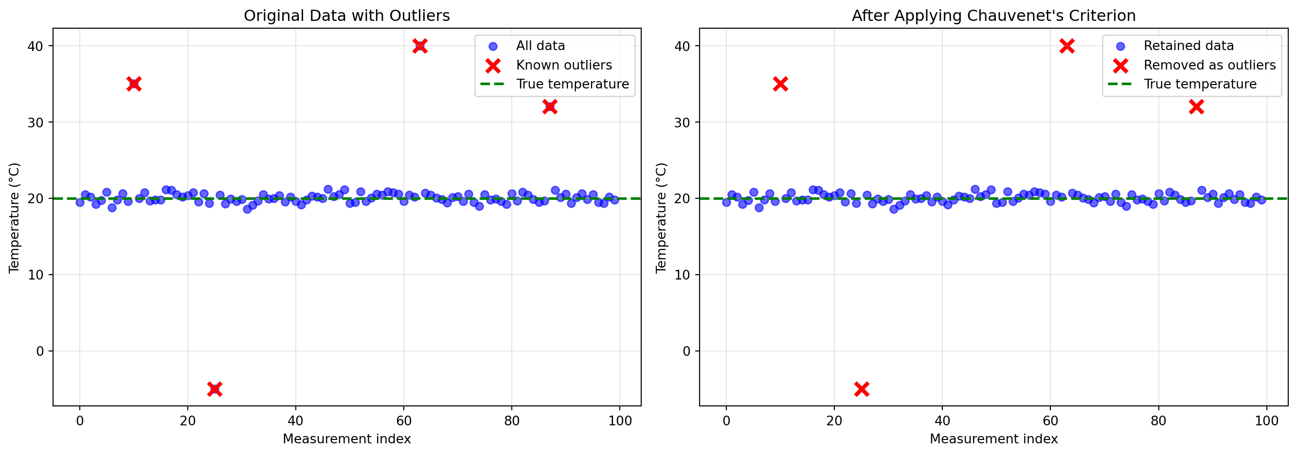
Statistical comparison:
Original data: mean=20.253, std=3.785
Cleaned data:  mean=20.034, std=0.569
True values:   mean=20.000, std=0.500
Key Observations:
Iteration matters: The first iteration might not catch all outliers because extreme outliers inflate the standard deviation. After removing the worst outliers, the standard deviation decreases, making remaining outliers more obvious.
Threshold selection: Using \(d_{threshold} = 3\) (3-sigma rule) is conservative and appropriate when you want to minimize false rejections. For noisier data or when outliers are more subtle, you might use a lower threshold like 2.5.
Performance: In this example, Chauvenet’s criterion successfully identified all four artificially injected outliers, and the cleaned data has statistics much closer to the true values.
Limitations:
- Assumes outliers are few (< 10-20% of data). With many outliers, the method can fail.
- Requires roughly Gaussian distribution of valid data
- Can’t distinguish between “bad outliers” (sensor errors) and “good outliers” (real extreme events)
4.2.3.6.4 When to Use Chauvenet’s Criterion
Good for:
- Cleaning sensor data before modeling
- Quality control in data collection
- Preprocessing for regression or averaging
- Small to moderate numbers of outliers (<10-20%)
Not good for:
- Anomaly detection (when outliers are the goal)
- Highly skewed or non-Gaussian data
- Data with many outliers (>20%)
- Time series with trends (detrend first!)
4.2.4 Estimating Trends in Time Series Data
Up to now, we’ve focused on understanding individual measurements and their uncertainties. But when collecting time series data from sensors, we typically want to understand patterns over time—trends, cycles, and relationships.
4.2.4.1 From Individual Points to Patterns
The simplest approach to estimating a physical quantity \(q_k\) at time \(t_i\) would be to just use the measurement at that time: \(\hat{q}_k(t_i) = y_{k,i}\). But this has serious limitations:
Problem 1: We can’t predict beyond our measurements
What if we want to estimate \(q\) at a time when we didn’t take a measurement? Or forecast future values? A single-point estimate gives us no predictive power.
Problem 2: We ignore structure
Most physical quantities don’t jump randomly—they follow patterns:
- Bridge deflection varies smoothly with load
- Temperature follows daily and seasonal cycles
- Water levels change gradually (except during storms)
If we believe the quantity has structure (smoothness, trends, periodicities), we should use that information!
Problem 3: We don’t leverage multiple measurements
If we have measurements at times \(t_1, t_2, \ldots, t_N\), and we believe the quantity varies smoothly, then nearby measurements should inform our estimate at time \(t_i\). Using only \(y_i\) wastes information from neighboring points.
4.2.4.2 The Core Idea: Model the Trend
Instead of treating each measurement independently, we’ll fit a model that describes how the physical quantity varies over time:
\[q(t) = f(t; \boldsymbol{\theta})\]
where:
- \(f\) is a function we choose (linear, polynomial, periodic, etc.)
- \(\boldsymbol{\theta}\) are parameters we estimate from data
Then we’ll find the parameters \(\boldsymbol{\theta}\) that best explain all our measurements \(y_1, y_2, \ldots, y_N\).
This approach has powerful benefits:
- Interpolation: Estimate \(q(t)\) at times between measurements
- Extrapolation: Predict \(q(t)\) at future times (with caution!)
- Noise reduction: The model “smooths out” measurement noise
- Compression: Store the model parameters instead of all raw data
- Insight: The model reveals underlying patterns
The simplest and most widely used method for fitting such models is linear regression.
4.2.4.3 Linear Regression: Finding the Best-Fit Line
Linear regression is one of the most fundamental tools in data analysis. Let’s build it from first principles, emphasizing the role of residuals—the key to understanding what regression is really doing.
4.2.4.3.1 The Setup: Simple Linear Regression
Suppose we have \(N\) measurements \((t_1, y_1), (t_2, y_2), \ldots, (t_N, y_N)\), and we believe the underlying physical quantity varies linearly with time:
\[q(t) = \beta_0 + \beta_1 t\]
where \(\beta_0\) is the intercept and \(\beta_1\) is the slope—these are the parameters we need to estimate.
Our measurements are noisy versions of this linear trend:
\[y_i = \beta_0 + \beta_1 t_i + n_i\]
Goal: Find the “best” values of \(\beta_0\) and \(\beta_1\) given our measurements.
4.2.4.3.2 Residuals: The Heart of Regression
For any choice of \(\beta_0\) and \(\beta_1\), we can compute the predicted value at time \(t_i\):
\[\hat{y}_i = \beta_0 + \beta_1 t_i\]
The residual \(r_i\) is the difference between the actual measurement and our prediction:
\[r_i = y_i - \hat{y}_i = y_i - (\beta_0 + \beta_1 t_i)\]
Key intuition:
- If our model is perfect and noise-free, all residuals would be zero
- In reality, residuals capture both measurement noise and model mismatch
- If the model structure is correct, residuals estimate the noise
- If the model structure is wrong, residuals include both noise and systematic error
4.2.4.3.3 The Least Squares Criterion
How do we choose the “best” \(\beta_0\) and \(\beta_1\)? We want to minimize the residuals, but some will be positive and some negative. A natural choice is to minimize the sum of squared residuals (also called the sum of squared errors, SSE):
\[\text{SSE}(\beta_0, \beta_1) = \sum_{i=1}^{N} r_i^2 = \sum_{i=1}^{N} (y_i - \beta_0 - \beta_1 t_i)^2\]
Why squares?
- Squares are always positive (can’t cancel out)
- Squares penalize large errors more than small ones
- Squaring leads to a smooth optimization problem with a unique solution
- Connects to maximum likelihood: Under Gaussian noise, minimizing SSE is equivalent to maximum likelihood estimation
4.2.4.3.4 Deriving the Solution
To find the minimum, we take derivatives with respect to \(\beta_0\) and \(\beta_1\) and set them equal to zero:
\[\frac{\partial \text{SSE}}{\partial \beta_0} = -2 \sum_{i=1}^{N} (y_i - \beta_0 - \beta_1 t_i) = 0\]
\[\frac{\partial \text{SSE}}{\partial \beta_1} = -2 \sum_{i=1}^{N} t_i(y_i - \beta_0 - \beta_1 t_i) = 0\]
Simplifying the first equation: \[\sum_{i=1}^{N} y_i = N\beta_0 + \beta_1 \sum_{i=1}^{N} t_i\]
\[\beta_0 = \bar{y} - \beta_1 \bar{t}\]
where \(\bar{y} = \frac{1}{N}\sum_i y_i\) and \(\bar{t} = \frac{1}{N}\sum_i t_i\).
Insight: The regression line always passes through the point \((\bar{t}, \bar{y})\)—the center of the data cloud.
Substituting this into the second equation and simplifying (algebra omitted for brevity):
\[\beta_1 = \frac{\sum_{i=1}^{N} (t_i - \bar{t})(y_i - \bar{y})}{\sum_{i=1}^{N} (t_i - \bar{t})^2} = \frac{\text{Cov}(t, y)}{\text{Var}(t)}\]
These are the least squares estimates for the slope and intercept.
4.2.4.3.5 Example: Fitting a Trend
Code
import numpy as np
import matplotlib.pyplot as plt

# Generate synthetic data with a linear trend plus noise
np.random.seed(42)
N = 30
t = np.linspace(0, 10, N)
beta_0_true = 5.0
beta_1_true = 2.0
noise_std = 3.0

y = beta_0_true + beta_1_true * t + np.random.normal(0, noise_std, N)

# Compute least squares estimates
t_bar = np.mean(t)
y_bar = np.mean(y)
beta_1 = np.sum((t - t_bar) * (y - y_bar)) / np.sum((t - t_bar)**2)
beta_0 = y_bar - beta_1 * t_bar

# Predictions and residuals
y_pred = beta_0 + beta_1 * t
residuals = y - y_pred

# Plot
fig, axes = plt.subplots(1, 2, figsize=(14, 5))

# Left plot: Data and fit
axes[0].scatter(t, y, alpha=0.6, s=50, label='Measurements', color='blue')
axes[0].plot(t, y_pred, 'r-', linewidth=2, label=f'Fit: y = {beta_0:.2f} + {beta_1:.2f}t')
axes[0].plot(t, beta_0_true + beta_1_true * t, 'g--', linewidth=2, alpha=0.7,
             label=f'True: y = {beta_0_true:.2f} + {beta_1_true:.2f}t')

# Draw residual lines
for i in range(N):
    axes[0].plot([t[i], t[i]], [y[i], y_pred[i]], 'k-', alpha=0.3, linewidth=1)

axes[0].scatter([t_bar], [y_bar], s=200, marker='X', color='red',
                edgecolors='black', linewidths=2, label='Centroid', zorder=5)
axes[0].set_xlabel('Time')
axes[0].set_ylabel('Measurement')
axes[0].set_title('Linear Regression Fit')
axes[0].legend()
axes[0].grid(True, alpha=0.3)

# Right plot: Residuals
axes[1].scatter(t, residuals, alpha=0.6, s=50, color='orange')
axes[1].axhline(0, color='red', linestyle='--', linewidth=2, label='Zero residual')
axes[1].set_xlabel('Time')
axes[1].set_ylabel('Residual (y - ŷ)')
axes[1].set_title(f'Residuals (SSE = {np.sum(residuals**2):.2f})')
axes[1].legend()
axes[1].grid(True, alpha=0.3)

plt.tight_layout()
plt.show()

print(f"True parameters: β₀ = {beta_0_true:.3f}, β₁ = {beta_1_true:.3f}")
print(f"Estimated parameters: β₀ = {beta_0:.3f}, β₁ = {beta_1:.3f}")
print(f"Residual standard deviation: {np.std(residuals, ddof=2):.3f}")
print(f"(Compare to true noise std: {noise_std:.3f})")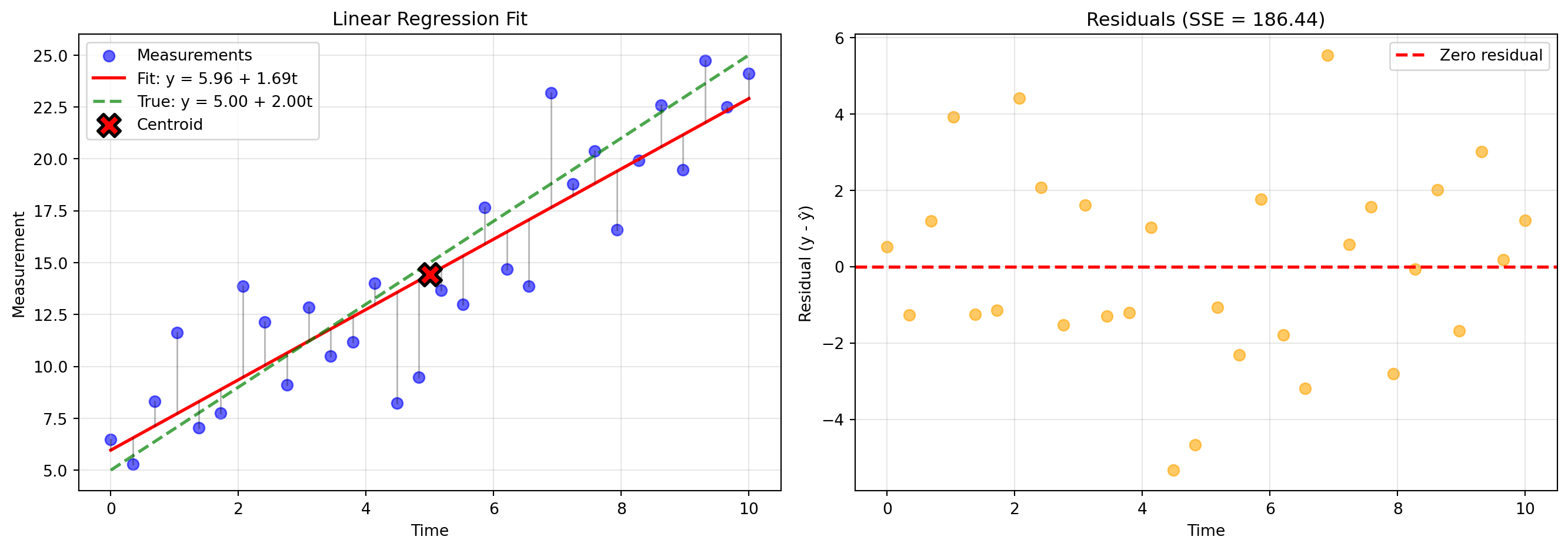
True parameters: β₀ = 5.000, β₁ = 2.000
Estimated parameters: β₀ = 5.964, β₁ = 1.694
Residual standard deviation: 2.580
(Compare to true noise std: 3.000)
Key observations:
- The fit line passes through the centroid (marked with X)
- Residuals scatter randomly around zero (if the model is correct)
- The residual standard deviation estimates the noise level
- Vertical lines show each residual—these are what we minimize in sum-of-squares
4.2.4.3.6 Using Regression for Outlier Detection
Remember Chauvenet’s criterion? We can combine it with regression for cleaning data with trends:
Iterative regression-based outlier removal:
- Fit a regression model to all data
- Compute residuals: \(r_i = y_i - \hat{y}_i\)
- Compute mean and std of residuals: \(\bar{r}\) and \(s_r\)
- Remove points where \(|r_i - \bar{r}|/s_r > d_{threshold}\)
- Refit the model and repeat until convergence
This is more appropriate than removing outliers based on raw \(y\) values when data has a trend, because we care about deviations from the expected trend, not from a constant mean.
4.2.4.3.7 Extension to Non-Linear Functions: The Power of Linearity in Parameters
Here’s a remarkable fact: linear regression can fit non-linear functions, as long as the function is linear in the parameters.
For example, suppose we believe our quantity follows a quadratic trend:
\[q(t) = \beta_0 + \beta_1 t + \beta_2 t^2\]
This looks non-linear (there’s a \(t^2\) term!), but it’s linear in the parameters \(\beta_0, \beta_1, \beta_2\). We can still use least squares!
Matrix Form: Define “basis functions” \(\phi_1(t), \phi_2(t), \ldots, \phi_M(t)\) and write:
\[q(t) = \sum_{j=1}^{M} \beta_j \phi_j(t) = \boldsymbol{\phi}(t)^T \boldsymbol{\beta}\]
For our quadratic example: \(\phi_1(t) = 1\), \(\phi_2(t) = t\), \(\phi_3(t) = t^2\).
With measurements \(y_1, \ldots, y_N\) at times \(t_1, \ldots, t_N\), construct the design matrix:
\[\mathbf{X} = \begin{bmatrix} \phi_1(t_1) & \phi_2(t_1) & \cdots & \phi_M(t_1) \\ \phi_1(t_2) & \phi_2(t_2) & \cdots & \phi_M(t_2) \\ \vdots & \vdots & \ddots & \vdots \\ \phi_1(t_N) & \phi_2(t_N) & \cdots & \phi_M(t_N) \end{bmatrix}\]
And the measurement vector: \(\mathbf{y} = [y_1, y_2, \ldots, y_N]^T\)
The least squares solution is:
\[\boldsymbol{\hat{\beta}} = (\mathbf{X}^T \mathbf{X})^{-1} \mathbf{X}^T \mathbf{y}\]
This single formula solves linear regression for:
- Polynomials: \(\phi_j(t) = t^{j-1}\)
- Fourier series: \(\phi_j(t) = \sin(j\omega t), \cos(j\omega t)\)
- Exponentials: \(\phi_j(t) = e^{\lambda_j t}\)
- Any combination you can imagine!
The key restriction: The model must be linear in the parameters \(\beta_j\), even if it’s non-linear in \(t\).
4.2.4.3.8 Example: Fitting a Polynomial
Code
# Generate data with a non-linear trend
np.random.seed(123)
N = 30
t = np.linspace(0, 5, N)
y_true = 2 + 3*t - 0.5*t**2  # Quadratic trend
y = y_true + np.random.normal(0, 2, N)

# Fit polynomials of degree 1, 2, and 3
degrees = [1, 2, 3]
colors = ['red', 'green', 'blue']

plt.figure(figsize=(10, 6))
plt.scatter(t, y, alpha=0.6, s=50, label='Measurements', color='black', zorder=5)

t_smooth = np.linspace(0, 5, 200)

for degree, color in zip(degrees, colors):
    # Construct design matrix
    X = np.column_stack([t**j for j in range(degree + 1)])
    X_smooth = np.column_stack([t_smooth**j for j in range(degree + 1)])

    # Least squares solution
    beta = np.linalg.solve(X.T @ X, X.T @ y)

    # Predictions
    y_pred = X @ beta
    y_smooth = X_smooth @ beta

    # Plot
    plt.plot(t_smooth, y_smooth, color=color, linewidth=2,
             label=f'Degree {degree} (SSE={np.sum((y - y_pred)**2):.1f})')

plt.xlabel('Time')
plt.ylabel('Measurement')
plt.title('Polynomial Regression: Different Model Complexities')
plt.legend()
plt.grid(True, alpha=0.3)
plt.tight_layout()
plt.show()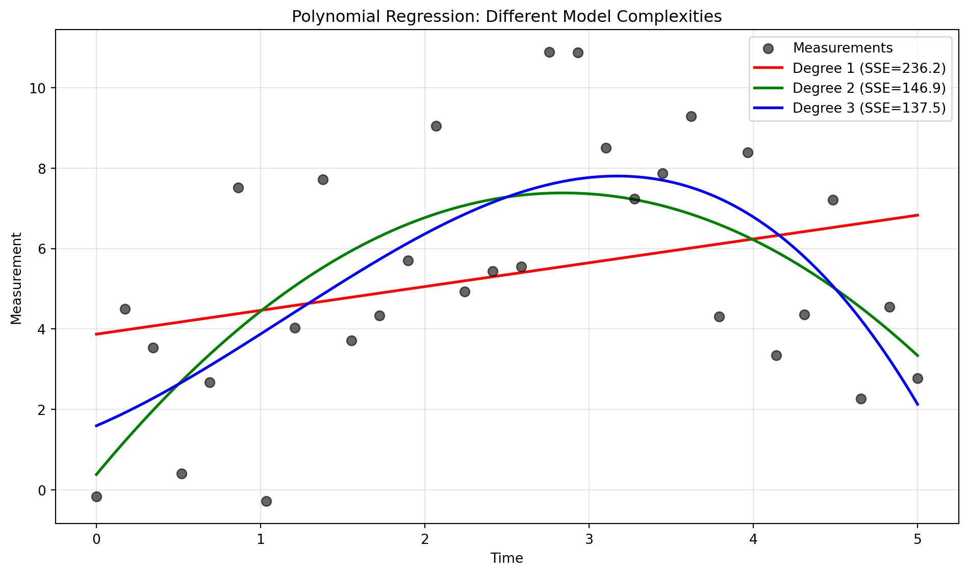
Important lessons:
- Degree 1 (linear) underfits—it can’t capture the curvature
- Degree 2 (quadratic) fits well—it matches the true model
- Degree 3 (cubic) fits slightly better (lower SSE) but starts to wiggle unnecessarily
This illustrates the bias-variance tradeoff:
- Too simple models have high bias (systematic error)
- Too complex models have high variance (overfitting to noise)
- The “just right” model matches the true complexity
4.2.4.3.9 Summary: The Power of Linear Regression
Linear regression is remarkably versatile:
- Simple and interpretable: Clear parameters with physical meaning
- Computationally efficient: Closed-form solution, no iterative optimization
- Extensible: Works for polynomials, Fourier series, and many non-linear basis functions
- Foundation for advanced methods: Underlies many machine learning algorithms
Key takeaways:
- Residuals are the difference between data and model predictions
- Good models have residuals that look like random noise
- Least squares minimizes the sum of squared residuals
- Linear regression works for non-linear functions (as long as they’re linear in parameters)
- Can be combined with outlier detection for robust fitting