import cvxpy as cp
import numpy as np

# Problem parameters
N = 24  # Prediction horizon (number of timesteps)

# Define optimization variables
T = cp.Variable(N + 1)    # Temperature at each timestep [T_0, T_1, ..., T_N]
u_kW = cp.Variable(N) # Control inputs in kW [u_0, u_1, ..., u_{N-1}]11 Basics of Control Theory for Buildings and Their Application
11.1 Lecture Overview
11.2 Introduction to Control Theory
Every physical system in a building — thermal, lighting, acoustic, hydraulic — has its own natural dynamics that tend toward an equilibrium determined by the environment and the laws of physics. Without intervention, indoor air temperature drifts toward the outdoor temperature, light levels follow the sun’s position and cloud cover, CO\(_2\) concentration rises with occupancy, and domestic hot water cools to ambient. In virtually every case, these natural equilibria are not where we want the building to operate. Occupants need temperatures around 21°C regardless of whether it’s \(-10°C\) or \(35°C\) outside, consistent illumination for visual tasks, acceptable air quality, and hot water on demand. Bridging the gap between where physics takes the system and where we need it to be requires actively expending energy — and doing so intelligently is the domain of control theory.
The challenge is that the objectives we care about often compete. Maintaining tight temperature control requires more energy than allowing wider fluctuations. Pre-cooling a building to reduce peak demand may temporarily sacrifice comfort. Ventilating aggressively for air quality increases heating or cooling loads. These trade-offs mean that building control is not simply a matter of turning equipment on and off — it requires balancing multiple, sometimes conflicting goals:
- Thermal comfort: Maintain indoor air temperature (and humidity, radiant temperature) within acceptable ranges
- Energy efficiency: Minimize total energy consumption or cost
- Indoor air quality: Keep CO\(_2\), particulate matter, and VOC concentrations below thresholds
- Visual comfort: Provide adequate and glare-free illumination
- Acoustic comfort: Manage noise from HVAC equipment and other sources
- Peak demand management: Reduce electricity demand during expensive or grid-stressed periods
- Equipment longevity: Avoid excessive cycling or operation outside design conditions
In the preceding lectures, we built up the physical understanding needed to model these systems — thermal dynamics via RC networks, electrical power fundamentals, and sensor/actuator technologies. Now we turn to the question: given a model of how the building behaves and a set of objectives, how do we make optimal control decisions?
11.2.1 Branches of Control Theory
At the broadest level, control strategies for buildings fall into two categories: passive and active. Passive control requires no energy input or real-time decision-making — it is designed into the building itself. Examples include high-performance insulation, thermal mass that buffers temperature swings, fixed shading devices sized for the sun’s seasonal path, and natural ventilation driven by stack effect or wind pressure. Passive strategies are powerful and should always be the first line of defense, but they have limits: they cannot adapt to changing conditions or occupant preferences, and they alone are rarely sufficient to maintain the precise indoor conditions modern buildings demand.
Active control bridges the gap by using energy and information to manipulate building systems in real time. Within active control, the simplest approach is open-loop control, where the system follows a pre-determined schedule with no knowledge of the current state. A time-clock that turns the HVAC system on at 6 AM and off at 6 PM is open-loop: it executes the same plan regardless of whether the building is already warm, whether it’s occupied, or whether the weather has changed. Open-loop control is easy to implement but inherently blind to what is actually happening in the building.
Sensor-based control improves on this by using measurements to inform decisions. Here the controller has access to some observation of the system’s state — a thermostat reading, a CO\(_2\) sensor, an occupancy detector — and adjusts its actions accordingly. Sensor-based control can be further divided by what information the controller uses. Feedback control reacts to the current (or recent) state of the system: the classic thermostat measures indoor temperature and turns heating on or off to correct deviations from the setpoint. Feedforward control, by contrast, anticipates disturbances before they affect the system: a controller that pre-heats a building based on a weather forecast or pre-cools before an anticipated occupancy surge is using feedforward information. In practice, most effective building controllers combine both — using feedback to correct for current errors and feedforward to anticipate known future disturbances.
Within sensor-based control, the question of how to design the control law — what action to take given the available information — has given rise to a rich landscape of approaches. Classical control (PID controllers, on-off thermostats) relies on simple rules and tuning. Modern control theory introduces state-space models and systematic design methods. Optimal control, which we focus on next, takes the approach of explicitly defining what “good” performance means through a cost function and then finding the control strategy that minimizes that cost — subject to the system’s dynamics and constraints.
11.2.2 Optimal Control and Its Place in Control Theory
The approaches described above — PID controllers, on-off thermostats, scheduled setbacks — are designed by intuition and tuning. They work well for simple cases, but as objectives multiply and constraints tighten, hand-crafted rules become difficult to design and impossible to guarantee as optimal. Optimal control takes a fundamentally different approach: instead of prescribing how the controller should behave, we define what we want (through a cost function) and what’s possible (through a model and constraints), and then let mathematical optimization find the best control strategy.
This requires formalizing the control problem with four ingredients:
1. Dynamical system — The physical process we are controlling, described by how its state evolves over time:
\[\dot{x}(t) = f(x(t), u(t), w_d(t))\]
where \(x(t)\) is the state vector (e.g., zone temperatures, wall temperatures, stored energy), \(u(t)\) is the control input vector (e.g., heating power, valve positions, fan speeds), and \(w_d(t)\) is a disturbance vector (e.g., outdoor temperature, solar radiation, internal heat gains from occupants and equipment). The function \(f\) encodes the physics — for thermal systems, these are the RC network equations we developed in earlier lectures.
2. Observations — What the controller can actually measure:
\[y(t) = g(x(t), u(t), w_n(t))\]
where \(y(t)\) is the observation vector (sensor readings) and \(w_n(t)\) is measurement noise. In general, the controller does not have direct access to the full state \(x\) — it only sees \(y\), which may be a noisy, incomplete view. For instance, we might measure indoor air temperature at one location but not the temperature distribution throughout the zone or within the walls.
3. Control law — The rule that maps available information to control actions:
\[u(t) = k(y(t), w_r(t))\]
where \(w_r(t)\) is a reference signal (e.g., the desired setpoint trajectory or an occupancy schedule). The function \(k\) is what we are designing — it is the controller itself.
4. Cost functional — A scalar measure of how well the controller performs over time:
\[J = \int_0^T \ell(x(t), u(t), w_r(t)) \, dt\]
where \(\ell\) is a stage cost that penalizes undesirable states (discomfort, high energy use, constraint violations) at each instant. The optimal control problem is then: find the control law \(k\) that minimizes \(J\) subject to the dynamics, observations, and constraints.
This framework is a natural fit for buildings. The competing objectives we identified — comfort, energy, air quality, cost — are encoded in \(J\). Physical limitations (maximum heating capacity, temperature bounds, ventilation minimums) appear as constraints. The building’s thermal, electrical, and air quality dynamics appear in \(f\). And the imperfect information available from sensors appears in \(g\) and \(w_n\). Among the various methods for solving optimal control problems, Model Predictive Control (MPC) has emerged as the most practical and widely used approach for buildings, and it is the focus of the remainder of this lecture.
11.3 Model Predictive Control Fundamentals
The optimal control framework above is elegant but, in its full generality, difficult to solve. Finding the globally optimal control law \(k\) over an infinite (or very long) time horizon, under uncertainty, for a constrained nonlinear system is computationally intractable for most practical problems. Model Predictive Control (MPC) offers a powerful and practical approximation that has become the dominant approach for optimal building control.
11.3.1 What is Model Predictive Control?
The core idea of MPC is to replace the intractable infinite-horizon problem with a sequence of tractable finite-horizon problems. At each control time step, the controller uses a model of the system to predict how the state will evolve over a fixed prediction horizon (e.g., the next 2–6 hours). It then solves an optimization problem to find the sequence of control inputs over that horizon that minimizes the cost function while satisfying all constraints. Crucially, only the first control action from the optimal sequence is actually applied to the system. At the next time step, the controller takes a new measurement, shifts the horizon forward by one step, and solves the optimization again. This strategy is called the receding horizon (or moving horizon) principle.
The receding horizon approach is what makes MPC robust in practice. Because the controller re-solves with fresh measurements at every step, it naturally corrects for model inaccuracies, unmeasured disturbances, and forecast errors. The model does not need to be perfect — it only needs to be good enough to make useful predictions over the horizon length. If the outdoor temperature turns out to be 2°C colder than forecasted, the controller will see the resulting indoor temperature deviation at the next measurement and adjust its plan accordingly.
MPC is particularly well suited to building control for several reasons. First, buildings have relatively slow dynamics — thermal time constants range from minutes to hours — so the optimization does not need to run at millisecond speeds; solving once every 5–15 minutes is typically sufficient. Second, forecast data that MPC needs is readily available: weather forecasts, occupancy schedules, and energy price signals can all be incorporated as predicted disturbances. Third, buildings have hard constraints that must be respected (equipment capacity limits, comfort bounds, ventilation minimums), and MPC handles these naturally as part of the optimization. Finally, the multi-objective nature of building control — balancing comfort, energy, cost, and emissions — maps directly onto MPC’s cost function, where each objective becomes a weighted term.
11.3.2 Components of an MPC Problem Formulation
Every MPC problem is defined by four ingredients: a cost functional that encodes what we want to achieve, constraints that encode what is physically and operationally possible, a dynamics model that predicts how the system will respond to our actions, and decision variables that define what the optimizer is free to choose. The choices we make for each of these determine the mathematical structure of the resulting optimization problem — and therefore what solution methods are available and how computationally expensive the problem is to solve.
11.3.2.1 Cost Functional (Objective Function)
The cost functional (also called the objective function) is the mathematical expression of “what good performance looks like.” It assigns a scalar cost to any candidate trajectory of states and control inputs over the prediction horizon, and the optimizer seeks the trajectory that minimizes this cost.
For building control, common cost functional forms include:
- Quadratic setpoint tracking: \(\sum_k w_{comfort}(T_i^k - T_{set})^2\) — penalizes deviations from a desired setpoint, with squared terms ensuring that large deviations are penalized disproportionately more than small ones
- Energy minimization: \(\sum_k w_{energy}(P_{hea}^k)^2\) or \(\sum_k w_{energy} P_{hea}^k\) — penalizes control effort; the quadratic form discourages large spikes in power while the linear form penalizes total energy equally
- Economic cost: \(\sum_k c_k \cdot P_{hea}^k \cdot \Delta t\) — where \(c_k\) is a time-varying electricity price, encouraging load shifting to off-peak hours
- Peak demand reduction: \(w_{peak} \cdot \max_k P_{hea}^k\) — penalizes the maximum power draw, which is relevant for demand charge reduction
In practice, the cost functional is usually a weighted sum of several of these terms. The weights (\(w_{comfort}\), \(w_{energy}\), etc.) are design parameters that set the trade-off between competing objectives. Choosing these weights is one of the most consequential decisions in MPC design — they determine whether the controller prioritizes tight comfort, low energy, or economic savings.
11.3.2.2 Constraints
Constraints define the boundaries of what is feasible — both physically and operationally. They come in two forms. Equality constraints express relationships that must hold exactly, the most important being the dynamics equations themselves: \(x_{k+1} = A_d x_k + B_d u_k + E_d w_k\). These are structural — they ensure the optimizer’s predicted trajectory is consistent with the physics of the building. The initial condition (\(x_0 = x_{measured}\)) is also an equality constraint that anchors the prediction to the current state.
Inequality constraints express bounds that must not be violated. These include actuator limits (heating power between 0 and \(P_{max}\), valve positions between 0% and 100%), comfort bounds (indoor temperature between \(T_{min}\) and \(T_{max}\)), and operational limits (minimum ventilation rates, maximum ramp rates for equipment). In some formulations, comfort bounds are treated as soft constraints — meaning small violations are allowed but penalized in the cost function — rather than hard constraints. This is useful because hard comfort constraints can make the problem infeasible (e.g., if the building is far from the comfort range and the heating system lacks the capacity to reach it within one time step). Soft constraints maintain feasibility while still discouraging violations.
11.3.2.3 Dynamics Model
The dynamics model is what gives MPC its predictive power — it is what distinguishes MPC from reactive controllers like thermostats. The model allows the controller to answer “if I apply this sequence of control inputs over the next \(N\) time steps, what will the indoor temperature trajectory look like?” This predictive capability is what enables anticipatory behavior: pre-heating before a cold front, pre-cooling before peak pricing, or coasting on thermal mass when outdoor conditions are favorable.
For building thermal control, the RC network models we developed in Lectures 5 and 6 provide exactly the kind of model MPC needs. Expressed in discrete-time state-space form (\(x_{k+1} = A_d x_k + B_d u_k + E_d w_k\)), they are linear, computationally cheap to evaluate, and have parameters with physical meaning. The trade-off is between model fidelity and computational cost: a 1R1C model is fast to solve but may not capture multi-zone interactions, while a higher-order model (3R3C, or even a full-building EnergyPlus model) is more accurate but makes the optimization harder. For MPC, a simpler model that captures the dominant dynamics is often preferable to a detailed model that slows down the optimization, since MPC’s receding horizon naturally compensates for model errors at each time step.
11.3.2.4 Decision Variables
The decision variables are the quantities the optimizer is free to choose in order to minimize the cost function. In a standard MPC formulation, these are the future control inputs \(u_0, u_1, \ldots, u_{N-1}\) over the prediction horizon. In many formulations (including the one we’ll use), the future states \(x_1, x_2, \ldots, x_N\) are also treated as decision variables, with the dynamics equations imposed as equality constraints linking them to the inputs. This “simultaneous” approach makes the optimization problem larger but keeps it structured in a way that modern solvers handle efficiently.
The prediction horizon \(N\) (expressed in number of time steps) determines how far into the future the controller plans. A longer horizon allows the controller to anticipate disturbances further ahead — for example, pre-heating overnight in anticipation of a cold morning — but increases the number of decision variables and thus the computational cost. For building thermal control with 15-minute time steps, horizons of 4–24 hours (16–96 steps) are typical. Beyond a certain point, extending the horizon yields diminishing returns because forecast accuracy degrades and the receding horizon re-solves the problem at every step anyway.
11.3.3 From Problem Formulation to Optimization Type
The choices made in the four components above — cost functional, constraints, dynamics, and decision variables — collectively determine the mathematical class of the resulting optimization problem. This matters enormously in practice because the problem class dictates what solution algorithms are available, how fast they run, and what guarantees they provide about the quality of the solution.
11.3.3.1 Linear vs. Nonlinear Problems
If the dynamics model is linear (as with our RC thermal networks), the constraints are linear inequalities (box bounds on temperatures and control inputs), and the cost function is linear, the MPC problem is a Linear Program (LP). If the cost is quadratic (e.g., squared deviation from setpoint), we get a Quadratic Program (QP). Both LPs and QPs can be solved reliably and efficiently by mature solvers — even for problems with thousands of variables, solutions typically take milliseconds to seconds.
When the dynamics are nonlinear (e.g., a detailed model that includes radiative heat exchange, humidity-dependent properties, or variable-speed equipment curves), the resulting optimization is a Nonlinear Program (NLP). NLPs are harder to solve: they require iterative algorithms (e.g., interior point methods, sequential quadratic programming), may take longer to converge, and — as we discuss next — may not guarantee a globally optimal solution. For building MPC, this is a key motivation for using linearized RC models even when more detailed nonlinear models are available: keeping the dynamics linear keeps the optimization tractable.
11.3.3.2 Convex vs. Non-Convex Problems
A problem is convex if the cost function is convex (bowl-shaped) and the feasible region defined by the constraints is a convex set. The critical property of convex problems is that any local minimum is also the global minimum — so if a solver finds a solution, it is guaranteed to be the best one. There are no hidden, better solutions lurking elsewhere in the feasible space.
QPs with linear constraints — which is what we get from linear RC models with quadratic comfort and energy costs — are convex. This is the practical sweet spot for building MPC: expressive enough to capture meaningful trade-offs (quadratic costs penalize large deviations more than small ones), yet convex enough that solvers can find the global optimum quickly and reliably. Tools like cvxpy (which we’ll use shortly) are specifically designed for convex problems and will even verify that your problem formulation is convex before attempting to solve it. Non-convex problems, by contrast, may have multiple local minima, and solvers can get trapped in a suboptimal one with no way to know whether a better solution exists.
11.3.3.3 Continuous vs. Discrete Decision Variables
In the formulations above, all decision variables are continuous — heating power can take any value between 0 and \(P_{max}\). But some building systems have inherently discrete decisions: a boiler is either on or off, a chiller plant has 1, 2, or 3 units running, a window is open or closed, and lighting may only be dimmable in fixed steps. When some decision variables are restricted to integer or binary values while others remain continuous, the result is a Mixed-Integer Program (MIP) — either a Mixed-Integer Linear Program (MILP) or Mixed-Integer Quadratic Program (MIQP) depending on the cost function.
MIPs are significantly harder to solve than their continuous counterparts. The discrete variables create a combinatorial explosion: with \(n\) binary variables, there are \(2^n\) possible combinations to consider. While modern MIP solvers (e.g., Gurobi, CPLEX) use branch-and-bound algorithms that avoid enumerating all combinations, solve times can still be orders of magnitude longer than for continuous QPs. For building MPC, this means that formulations with many on/off decisions (e.g., coordinating a large number of discrete HVAC units) may push against real-time computation limits. A common workaround is to solve the continuous relaxation first (allowing “fractional” on/off values) and then round the result, accepting a small loss of optimality in exchange for computational tractability.
11.4 MPC for Building Thermal Dynamics
In Lectures 5 and 6, we developed thermal network models to represent how heat flows through buildings. We learned how to model walls, windows, and thermal mass using networks of resistances (R) and capacitances (C), deriving equations that describe the building’s thermal dynamics. Those models allowed us to predict what would happen to indoor temperature given certain inputs (outdoor temperature, solar gains, heating power). Now, we take the next step: using those same models not just for prediction, but for making optimal control decisions.
This is where Model Predictive Control comes in. MPC leverages a dynamics model (like our RC thermal networks) to predict the future behavior of the building over some time horizon. It then uses optimization to find the sequence of control inputs (e.g., heating/cooling power) that best achieves our objectives—such as maintaining comfort while minimizing energy consumption—subject to physical and operational constraints.
The beauty of MPC for building control is that it naturally handles several challenges that simple reactive controllers (like proportional controllers) struggle with:
- Anticipatory behavior: MPC can “see” upcoming disturbances (weather forecasts, occupancy schedules) and act proactively rather than just reacting to current conditions
- Multi-objective optimization: We can explicitly balance competing goals like comfort, energy cost, and peak demand reduction in a single cost function
- Constraint handling: Physical limits (maximum heating power, comfort temperature bounds) are directly incorporated as constraints in the optimization problem
- Thermal mass utilization: MPC can strategically use the building’s thermal mass to shift energy consumption to off-peak hours while maintaining comfort
The key insight is this: the RC thermal network models we’ve studied provide exactly the kind of predictive model MPC needs. Because these models are often linear (or can be linearized), we can formulate the resulting MPC problem as a convex optimization problem that can be solved efficiently and reliably at each control timestep.
11.4.1 Using RC Thermal Networks in MPC
To use RC thermal networks in an MPC framework, we need to express the building’s thermal dynamics in a form that’s compatible with optimization algorithms. Let’s recall that RC thermal networks give us differential equations describing how temperatures evolve over time. For example, a simple 1R1C network yields:
\[C\frac{dT_i}{dt} = \frac{1}{R}(T_a - T_i) + P_{hea}\]
where \(T_i\) is the indoor temperature, \(T_a\) is the ambient (outdoor) temperature, \(P_{hea}\) is the heating power, \(C\) is the thermal capacitance, and \(R\) is the thermal resistance.
For MPC, we need to transform this continuous-time differential equation into a form that:
- Separates states, inputs, and disturbances: We need to clearly distinguish what we control (inputs) from what we observe (states) and what affects us but we can’t control (disturbances)
- Works with discrete time steps: Digital controllers operate at discrete time intervals (e.g., every 15 minutes), so we need a discrete-time representation
- Enables prediction over a horizon: The model needs to let us predict future states based on sequences of future inputs and disturbances
The standard approach is to use state-space representation, which expresses the system dynamics in matrix form. This representation is ideal for MPC because:
- It provides a compact, general framework that works for networks of any complexity (1R1C, 2R2C, etc.)
- It clearly separates the system’s state evolution from the outputs we measure
- It interfaces naturally with optimization solvers that expect linear dynamics
- It makes it straightforward to incorporate forecasts (weather, occupancy, etc.)
11.4.2 State-Space Representation Review
The state-space representation is a mathematical framework for modeling dynamical systems. For linear systems, the continuous-time state-space form is:
\[\dot{x}(t) = Ax(t) + Bu(t) + Ew(t)\]
where:
- \(x(t)\) is the state vector (temperatures in our case, like \(T_i\), \(T_e\))
- \(u(t)\) is the control input vector (what we can manipulate, like \(P_{hea}\))
- \(w(t)\) is the disturbance vector (external factors we can’t control, like \(T_a\), solar irradiance)
- \(A\) is the state matrix (describes system dynamics)
- \(B\) is the input matrix (describes how control inputs affect states)
- \(E\) is the disturbance matrix (describes how disturbances affect states)
In Lecture 6, you saw how thermal network models could be written in this form. For example, the 2R2C model equations can be expressed as a 2×2 state matrix operating on the state vector \([T_i, T_e]^T\).
11.4.2.1 Discrete-Time State-Space Form
Since digital controllers operate at discrete time steps (not continuously), we need the discrete-time version. Using explicit Euler discretization with timestep \(\Delta t\), we get:
\[x_{k+1} = A_d x_k + B_d u_k + E_d w_k\]
where the subscript \(k\) denotes the time index (i.e., \(x_k = x(k \cdot \Delta t)\)), and the discrete-time matrices are related to the continuous-time ones by:
\[A_d = I + \Delta t \cdot A\] \[B_d = \Delta t \cdot B\] \[E_d = \Delta t \cdot E\]
This discrete-time form is exactly what we need for MPC: given the current state \(x_k\), future control inputs \(u_k, u_{k+1}, \ldots\), and forecasts of disturbances \(w_k, w_{k+1}, \ldots\), we can recursively predict future states \(x_{k+1}, x_{k+2}, \ldots\) over the MPC horizon.
NoteWhy Explicit Euler?
More sophisticated discretization methods (e.g., implicit Euler, Runge-Kutta) can provide better accuracy, especially for stiff systems or large timesteps. However, explicit Euler is simple, maintains linearity (which keeps the MPC problem convex), and is sufficiently accurate for typical building control timesteps (15-60 minutes). For the purposes of this course, we’ll use explicit Euler discretization.
11.4.3 Example: 1R1C Model for MPC
Let’s work through a complete example of formulating an MPC problem for a building represented by a simple 1R1C thermal network. This will illustrate all four components of MPC: the dynamic model, cost function, constraints, and optimization.
11.4.3.1 Model Setup
Consider a building modeled as a single thermal zone with:
- State: Indoor temperature \(T_i\) (the temperature we want to control)
- Control input: Heating power \(P_{hea}\) (what we manipulate)
- Disturbance: Ambient temperature \(T_a\) (outdoor temperature, which we forecast but can’t control)
The continuous-time thermal dynamics are:
\[C \frac{dT_i}{dt} = \frac{1}{R}(T_a - T_i) + P_{hea}\]
where \(C\) is the thermal capacitance [J/K] and \(R\) is the thermal resistance [K/W].
Rearranging into state-space form:
\[\frac{dT_i}{dt} = -\frac{1}{RC}T_i + \frac{1}{C}P_{hea} + \frac{1}{RC}T_a\]
This gives us:
- State matrix: \(A = -\frac{1}{RC}\)
- Input matrix: \(B = \frac{1}{C}\)
- Disturbance matrix: \(E = \frac{1}{RC}\)
Discrete-time version (using explicit Euler with timestep \(\Delta t\)):
\[T_i^{k+1} = T_i^k + \frac{\Delta t}{C}\left[\frac{1}{R}(T_a^k - T_i^k) + P_{hea}^k\right]\]
Rearranging to isolate \(T_i^{k+1}\):
\[T_i^{k+1} = \underbrace{\left(1 - \frac{\Delta t}{RC}\right)}_{a}T_i^k + \underbrace{\frac{\Delta t}{C}}_{b}P_{hea}^k + \underbrace{\frac{\Delta t}{RC}}_{e}T_a^k\]
or more compactly:
\[T_i^{k+1} = a \cdot T_i^k + b \cdot P_{hea}^k + e \cdot T_a^k\]
where \(a = 1 - \frac{\Delta t}{RC}\), \(b = \frac{\Delta t}{C}\), and \(e = \frac{\Delta t}{RC}\).
11.4.3.2 Cost Function Design
The MPC controller needs to balance two competing objectives:
- Comfort: Keep indoor temperature close to a setpoint \(T_{set}\)
- Energy efficiency: Minimize heating energy consumption
A typical cost function that balances these objectives is:
\[J = \sum_{k=0}^{N-1} \left[ w_{comfort} (T_i^k - T_{set})^2 + w_{energy} (P_{hea}^k)^2 \right]\]
where:
- \(N\) is the prediction horizon (number of timesteps into the future)
- \(w_{comfort}\) is the weight on comfort violations (large value = prioritize comfort)
- \(w_{energy}\) is the weight on energy use (large value = prioritize energy savings)
- Squared terms penalize large deviations more heavily than small ones
The ratio \(\frac{w_{comfort}}{w_{energy}}\) determines the trade-off:
- High ratio → tight temperature control, higher energy use
- Low ratio → looser temperature control, lower energy use
NoteTerminal Cost
In addition to the stage costs above, MPC formulations often include a terminal cost on the final state:
\[J = \sum_{k=0}^{N-1} \left[ w_{comfort} (T_i^k - T_{set})^2 + w_{energy} (P_{hea}^k)^2 \right] + w_{terminal}(T_i^N - T_{set})^2\]
The terminal cost serves several purposes:
- Stability: For certain choices of terminal cost and terminal constraints, the terminal cost can guarantee closed-loop stability of the MPC controller
- Long-term behavior: It encourages the controller to leave the system in a good state at the end of the horizon, which helps performance beyond the prediction horizon
- Approximation of infinite horizon: It approximates the cost-to-go from the terminal state onward when we can’t afford to optimize over an infinite horizon
For practical building control, the terminal cost is often set equal to or slightly higher than the stage comfort cost weight (i.e., \(w_{terminal} \geq w_{comfort}\)).
11.4.3.3 Constraint Specification
Real systems have physical and operational limits that must be respected:
Temperature comfort bounds:
\[T_{min} \leq T_i^k \leq T_{max} \quad \forall k = 1, \ldots, N\]
For example, \(T_{min} = 20°C\) and \(T_{max} = 24°C\) define an acceptable comfort range.
Heating power limits:
\[0 \leq P_{hea}^k \leq P_{max} \quad \forall k = 0, \ldots, N-1\]
where \(P_{max}\) is the maximum capacity of the heating system (e.g., 5000 W). Note that we typically don’t allow negative heating power (cooling would be a separate control input).
Initial condition:
\[T_i^0 = T_i^{measured}\]
The optimization must start from the current measured temperature.
11.4.3.4 Complete Problem Formulation
Putting it all together, the MPC optimization problem at each timestep is:
ImportantMPC Optimization Problem (1R1C Example)
Decision variables: \(T_i^0, T_i^1, \ldots, T_i^N\) and \(P_{hea}^0, P_{hea}^1, \ldots, P_{hea}^{N-1}\)
Minimize:
\[J = \sum_{k=0}^{N-1} \left[ w_{comfort} (T_i^k - T_{set})^2 + w_{energy} (P_{hea}^k)^2 \right] + w_{terminal}(T_i^N - T_{set})^2\]
Subject to:
Dynamics (for \(k = 0, \ldots, N-1\)):
\[T_i^{k+1} = a \cdot T_i^k + b \cdot P_{hea}^k + e \cdot T_a^k\]
Initial condition:
\[T_i^0 = T_i^{measured}\]
Temperature bounds (for \(k = 1, \ldots, N\)):
\[T_{min} \leq T_i^k \leq T_{max}\]
Heating power bounds (for \(k = 0, \ldots, N-1\)):
\[0 \leq P_{hea}^k \leq P_{max}\]
Key observations:
- This is a convex quadratic program (QP) because the cost is quadratic and all constraints are linear
- We have \(N+1\) temperature variables and \(N\) control variables (total: \(2N+1\) decision variables)
- Once solved, we implement only \(P_{hea}^0\) (the first control action) and discard the rest
- At the next timestep, we resolve the entire problem with updated measurements and forecasts—this is the receding horizon principle of MPC
11.5 Implementation with cvxpy
Now that we’ve formulated the MPC problem mathematically, we need a way to actually solve it. While we could implement our own optimization algorithms (gradient descent, interior point methods, etc.), this would be time-consuming and error-prone. Instead, we’ll use CVXPY, a Python library specifically designed for formulating and solving convex optimization problems.
11.5.1 What is cvxpy?
CVXPY (pronounced “cvx-pie”) is a domain-specific language for convex optimization embedded in Python. It allows you to express optimization problems in a natural mathematical syntax, then automatically transforms them into a standard form and dispatches them to appropriate solvers.
Key features that make cvxpy ideal for MPC:
- Declarative syntax: You write code that looks like the mathematical problem formulation
- Automatic problem classification: cvxpy determines whether your problem is linear, quadratic, convex, etc.
- Solver interface: Automatically selects and interfaces with appropriate solvers (OSQP, ECOS, SCS, etc.)
- Disciplined Convex Programming (DCP): Enforces rules that guarantee your problem is actually convex
- Fast prototyping: Quickly experiment with different cost functions and constraints
How cvxpy works:
- You define variables using
cp.Variable() - You express constraints using Python comparison operators (
<=,>=,==) - You define the objective using cvxpy functions like
cp.Minimize(),cp.sum_squares(), etc. - You create a problem object:
cp.Problem(objective, constraints) - You call
problem.solve()which invokes the appropriate solver - You extract the solution from the
.valueattribute of your variables
For our MPC application, cvxpy will handle all the complexity of transforming our problem into the standard form expected by quadratic programming (QP) solvers, and will efficiently solve the optimization at each control timestep.
11.5.2 Setting Up an MPC Problem in cvxpy
Let’s translate the 1R1C MPC problem from the previous section into cvxpy code. We’ll go step-by-step, mapping each mathematical element to its cvxpy equivalent.
Step 1: Define optimization variables
In our problem, the decision variables are the temperature trajectory and the control inputs:
Step 2: Set up constraint list
We’ll build a Python list to hold all constraints:
constraints = []Step 3: Add initial condition constraint
\[T_i^0 = T_i^{measured}\]
T_current = 20.0  # Current measured temperature [°C]
constraints += [T[0] == T_current]
Step 4: Add dynamics constraints
For each timestep \(k = 0, \ldots, N-1\):
\[T_i^{k+1} = a \cdot T_i^k + b \cdot P_{hea}^k + e \cdot T_a^k\]
# Model parameters (example values for a 1R1C model)
R = 0.005     # Thermal resistance [K/W]
C = 5e6       # Thermal capacitance [J/K]
dt = 900      # Timestep [seconds] (15 minutes)

# Compute discrete-time coefficients
a = 1 - dt/(R*C)
b = dt/C * 1000  # Multiplies kW, so scale by 1000
e = dt/(R*C)

# Ambient temperature forecast (assume constant for simplicity)
T_amb = np.full(N, 5.0)  # [°C]

# Add dynamics constraints for each timestep
for k in range(N):
    constraints += [T[k+1] == a*T[k] + b*u_kW[k] + e*T_amb[k]]
Step 5: Add temperature bounds
\[T_{min} \leq T_i^k \leq T_{max} \quad \forall k = 1, \ldots, N\]
T_min = 20.0  # Minimum comfort temperature [°C]
T_max = 24.0  # Maximum comfort temperature [°C]

constraints += [T[1:] >= T_min]  # Apply to T[1], T[2], ..., T[N]
constraints += [T[1:] <= T_max]
Step 6: Add control input bounds
\[0 \leq P_{hea}^k \leq P_{max} \quad \forall k = 0, \ldots, N-1\]
P_max_kW = 5.0  # Maximum heating power [kW]

constraints += [u_kW >= 0]
constraints += [u_kW <= P_max_kW]
Step 7: Define the cost function
\[J = \sum_{k=0}^{N-1} \left[ w_{comfort} (T_i^k - T_{set})^2 + w_{energy} (P_{hea}^k)^2 \right] + w_{terminal}(T_i^N - T_{set})^2\]
T_set = 21.0      # Temperature setpoint [°C]
w_comfort = 1.0   # Weight on comfort
w_energy = 0.01   # Weight on energy
w_terminal = 1.0  # Terminal cost weight

# Stage costs (over horizon)
comfort_cost = w_comfort * cp.sum_squares(T[:-1] - T_set)  # T[0] through T[N-1]
energy_cost = w_energy * cp.sum_squares(u_kW / P_max_kW)

# Terminal cost
terminal_cost = w_terminal * cp.sum_squares(T[-1] - T_set)  # T[N]

# Total cost
total_cost = comfort_cost + energy_cost + terminal_cost
Step 8: Create and solve the problem
# Define the optimization problem
problem = cp.Problem(cp.Minimize(total_cost), constraints)

# Solve the problem
problem.solve()

# Check if solution was found
if problem.status in ["optimal", "optimal_inaccurate"]:
    print(f"Optimal solution found!")
    print(f"Optimal cost: {problem.value:.2f}")
else:
    print(f"Optimization failed: {problem.status}")
Optimal solution found!
Optimal cost: 1.6111.5.3 Solving and Extracting Results
Once problem.solve() completes, the solution is stored in the .value attribute of each variable:
# Extract optimal temperature trajectory
T_optimal = T.value
print(f"Temperature trajectory: {T_optimal}")

# Extract optimal control sequence
u_optimal = u_kW.value
print(f"Control sequence (kW): {u_optimal}")

# MPC receding horizon: apply only the first control action
u_apply = u_optimal[0]
print(f"\nControl to apply now: {u_apply:.2f} kW")
Temperature trajectory: [20. 20.36 20.70704 20.99634105 20.99970444 20.99974354
20.999744 20.999744 20.999744 20.999744 20.999744 20.999744
20.999744 20.999744 20.999744 20.999744 20.999744 20.999744
20.999744 20.999744 20.999744 20.99974399 20.99974309 20.99966527
20.99297167]
Control sequence (kW): [5. 5. 4.74863604 3.21795373 3.20015812 3.19995123
3.19994883 3.1999488 3.1999488 3.1999488 3.1999488 3.1999488
3.1999488 3.1999488 3.1999488 3.1999488 3.1999488 3.1999488
3.1999488 3.1999488 3.19994874 3.19994377 3.19951629 3.16274642]
Control to apply now: 5.00 kWInterpreting the results:
problem.value: The optimal value of the cost functionproblem.status: Solution status (e.g., “optimal”, “infeasible”, “unbounded”)T.value: Array of optimal temperatures \([T_0, T_1, \ldots, T_N]\)u_kW.value: Array of optimal control inputs in kW \([u_0, u_1, \ldots, u_{N-1}]\)
Important notes:
- Check the status: Always verify that
problem.statusis “optimal” before using the solution - Receding horizon: In practice, you only implement
u_optimal[0], then re-solve the problem at the next timestep with new measurements - Solver selection: cvxpy automatically selects a solver, but you can specify one:
problem.solve(solver=cp.OSQP)
11.5.4 Complete Example: MPC Controller for 1R1C Model
Here’s a complete, runnable example that brings together everything we’ve discussed. This implements an MPC controller as a Python function that can be called repeatedly at each timestep:
import cvxpy as cp
import numpy as np
import matplotlib.pyplot as plt

def mpc_controller_1R1C(T_current, T_amb_forecast, params):
    """
    MPC controller for a 1R1C thermal model.

    Parameters
    ----------
    T_current : float
        Current measured indoor temperature [°C]
    T_amb_forecast : array
        Forecast of ambient temperature over horizon [°C]
    params : dict
        Dictionary containing:
        - 'R': Thermal resistance [K/W]
        - 'C': Thermal capacitance [J/K]
        - 'dt': Timestep [seconds]
        - 'N': Prediction horizon
        - 'T_set': Temperature setpoint [°C]
        - 'T_min': Minimum comfort temperature [°C]
        - 'T_max': Maximum comfort temperature [°C]
        - 'P_max_kW': Maximum heating power [kW]
        - 'w_comfort': Weight on comfort cost
        - 'w_energy': Weight on energy cost
        - 'w_terminal': Weight on terminal cost

    Returns
    -------
    u_optimal : array
        Optimal control sequence [kW]
    T_optimal : array
        Predicted temperature trajectory [°C]
    """
    # Extract parameters
    R = params['R']
    C = params['C']
    dt = params['dt']
    N = params['N']
    T_set = params['T_set']
    T_min = params['T_min']
    T_max = params['T_max']
    P_max_kW = params['P_max_kW']
    w_comfort = params['w_comfort']
    w_energy = params['w_energy']
    w_terminal = params['w_terminal']

    # Compute discrete-time model coefficients
    a = 1 - dt/(R*C)
    b = dt/C * 1000  # Multiplies kW, so scale by 1000
    e = dt/(R*C)

    # Define optimization variables
    T = cp.Variable(N + 1)
    u_kW = cp.Variable(N)

    # Build constraints
    constraints = []

    # Initial condition
    constraints += [T[0] == T_current]

    # Dynamics
    for k in range(N):
        constraints += [T[k+1] == a*T[k] + b*u_kW[k] + e*T_amb_forecast[k]]

    # Temperature bounds
    constraints += [T[1:] >= T_min]
    constraints += [T[1:] <= T_max]

    # Control bounds
    constraints += [u_kW >= 0]
    constraints += [u_kW <= P_max_kW]

    # Define cost function
    comfort_cost = w_comfort * cp.sum_squares(T[:-1] - T_set)
    energy_cost = w_energy * cp.sum_squares(u_kW / P_max_kW)
    terminal_cost = w_terminal * cp.sum_squares(T[-1] - T_set)
    total_cost = comfort_cost + energy_cost + terminal_cost

    # Solve
    problem = cp.Problem(cp.Minimize(total_cost), constraints)
    problem.solve(verbose=False)

    # Check solution status
    if problem.status not in ["optimal", "optimal_inaccurate"]:
        print(f"Warning: Optimization status = {problem.status}")
        return None, None

    return u_kW.value, T.value


# Model parameters (example values)
params = {
    'R': 0.005,         # [K/W]
    'C': 5e6,           # [J/K]
    'dt': 900,          # [s] = 15 minutes
    'N': 24,            # 24 steps = 6 hours ahead
    'T_set': 21.0,      # [°C]
    'T_min': 20.0,      # [°C]
    'T_max': 24.0,      # [°C]
    'P_max_kW': 5.0,    # [kW]
    'w_comfort': 1.0,
    'w_energy': 0.01,
    'w_terminal': 1.0
}

# Simulation setup
sim_hours = 24
sim_steps = int(sim_hours * 3600 / params['dt'])

# Generate ambient temperature profile (cold morning, warmer afternoon)
time_hours = np.linspace(0, sim_hours, sim_steps)
T_amb_actual = 5 + 8*np.sin(2*np.pi*(time_hours - 6)/24)  # [°C]

# Initialize state
T_current = 20.0  # Start at 20°C

# Storage for results
T_history = [T_current]
u_history = []

# MPC simulation loop
for step in range(sim_steps):
    # Create forecast (here we assume perfect forecast)
    forecast_end = min(step + params['N'], sim_steps)
    forecast_length = forecast_end - step
    T_amb_forecast = T_amb_actual[step:forecast_end]

    # Pad forecast if needed
    if forecast_length < params['N']:
        T_amb_forecast = np.concatenate([
            T_amb_forecast,
            np.full(params['N'] - forecast_length, T_amb_forecast[-1])
        ])

    # Solve MPC problem
    u_opt, T_pred = mpc_controller_1R1C(T_current, T_amb_forecast, params)

    if u_opt is None:
        print(f"MPC failed at step {step}")
        break

    # Apply first control action (receding horizon)
    u_apply = u_opt[0]
    u_history.append(u_apply)

    # Simulate actual system response (using same 1R1C model)
    a = 1 - params['dt']/(params['R']*params['C'])
    b = params['dt']/params['C'] * 1000  # u_apply is in kW
    e = params['dt']/(params['R']*params['C'])

    T_current = a*T_current + b*u_apply + e*T_amb_actual[step]
    T_history.append(T_current)

# Plot results
fig, (ax1, ax2) = plt.subplots(2, 1, figsize=(12, 8), sharex=True)

# Temperature plot
ax1.plot(time_hours, T_history[:-1], label='Indoor Temp', linewidth=2)
ax1.plot(time_hours, T_amb_actual, label='Outdoor Temp', linestyle='--', alpha=0.7)
ax1.axhline(params['T_set'], color='green', linestyle=':', label='Setpoint')
ax1.axhline(params['T_min'], color='red', linestyle=':', alpha=0.5, label='Comfort bounds')
ax1.axhline(params['T_max'], color='red', linestyle=':', alpha=0.5)
ax1.set_ylabel('Temperature [°C]')
ax1.legend()
ax1.grid(True, alpha=0.3)
ax1.set_title('MPC Controller Performance (1R1C Model)')

# Control input plot
ax2.plot(time_hours, u_history, label='Heating Power', linewidth=2, color='orange')
ax2.set_xlabel('Time [hours]')
ax2.set_ylabel('Heating Power [kW]')
ax2.legend()
ax2.grid(True, alpha=0.3)

plt.tight_layout()
plt.show()

# Print summary statistics
print(f"\nSimulation Summary:")
print(f"  Mean indoor temperature: {np.mean(T_history[:-1]):.2f} °C")
print(f"  Temperature std dev: {np.std(T_history[:-1]):.2f} °C")
print(f"  Total energy used: {np.sum(u_history)*params['dt']/3600:.2f} kWh")
print(f"  Average power: {np.mean(u_history):.2f} kW")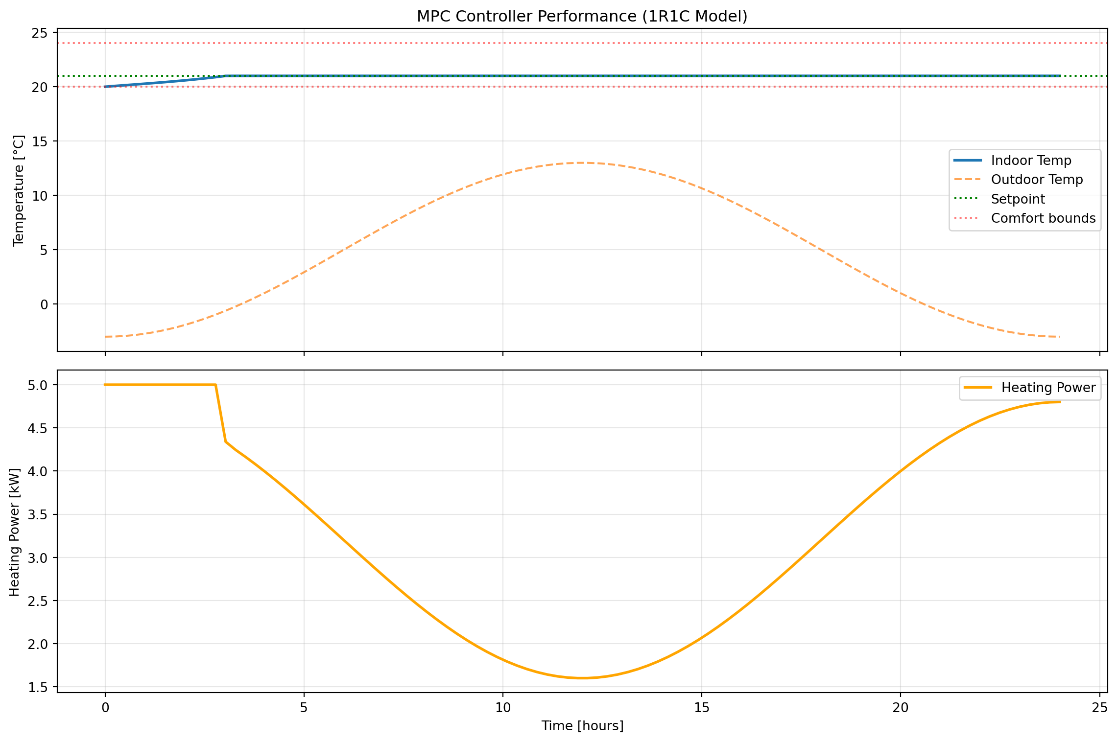
Simulation Summary:
  Mean indoor temperature: 20.93 °C
  Temperature std dev: 0.22 °C
  Total energy used: 78.23 kWh
  Average power: 3.26 kW
You can now re-run this to experiment with a few different things, including:
- Cost function weights (
w_comfort,w_energy) - Prediction horizon (
N) - Comfort bounds (
T_min,T_max) - Model parameters (
R,C)
11.6 Building Optimization Testing Framework (BOPTEST)
The MPC controller we developed in the previous section works well in simulation with our simple 1R1C model. But how would it perform in a real building with more complex dynamics, weather variations, and occupancy patterns? More importantly, how can we objectively compare different control strategies to determine which is best?
This is where BOPTEST (Building Optimization Testing Framework) comes in. BOPTEST provides a standardized platform for testing and benchmarking building control algorithms using realistic building simulations. Think of it as a “digital twin” testbed where you can evaluate your controller’s performance before deploying it to an actual building.
11.6.1 The Need for Standardized Benchmarking
Evaluating building control algorithms is challenging for several reasons:
Problem 1: Lack of reproducibility
- Different researchers test on different buildings with different characteristics
- Weather conditions, occupancy patterns, and baseline systems vary
- Results from one study can’t be directly compared to another
- “My controller saved 30% energy” is meaningless without context
Problem 2: Real-world deployment barriers
- Testing experimental controllers on real buildings is risky and expensive
- Building owners are reluctant to allow untested algorithms to control their HVAC
- Seasonal variations mean you might wait months to evaluate performance
- Safety and comfort constraints limit what experiments you can run
Problem 3: Fair comparison difficulties
- Even with the same building, comparing controllers requires identical conditions
- You can’t replay the exact same weather twice in a real building
- Baseline controller performance varies with tuning
- Implementation details (sampling rates, sensor noise) affect results
BOPTEST’s solution:
BOPTEST addresses these challenges by providing:
- Standardized test cases: Realistic building models representing different archetypes (residential, commercial, etc.)
- Reproducible conditions: Exact same weather, occupancy, and disturbances every time
- Fair comparison: All controllers tested on identical virtual buildings
- Comprehensive metrics: Standardized KPIs (energy, comfort, cost, emissions) for evaluation
- Open access: Free, open-source framework anyone can use
This enables apples-to-apples comparisons where the only variable is the control algorithm itself.
11.6.2 What is BOPTEST?
BOPTEST is an open-source software framework developed through an international collaboration (IBPSA Project 1) that provides:
Core Components:
- Building Emulators: High-fidelity building models implemented in Modelica (a physical modeling language)
- Models include detailed HVAC systems, envelope dynamics, occupancy, and weather
- Simulate at sub-minute timesteps for realistic response
- Include measurement noise and actuator dynamics
- REST API: Standard web-based interface for controller interaction
- Controllers send control signals via HTTP requests
- Receive measurements and forecasts in response
- Language-agnostic (works with Python, MATLAB, Julia, etc.)
- KPI Calculation Engine: Automatic computation of performance metrics
- Energy consumption (heating, cooling, total)
- Thermal comfort violations (PMV, operative temperature)
- Economic cost (based on time-of-use pricing)
- CO₂ emissions
How it works:
┌─────────────────┐         HTTP/REST API        ┌──────────────────┐
│  Your Control   │◄────────────────────────────►│ BOPTEST Service  │
│   Algorithm     │  - Send control inputs       │  (Building Model)│
│  (Python/etc.)  │  - Get measurements          │   + KPI tracker  │
└─────────────────┘  - Get forecasts             └──────────────────┘
The controller you develop runs independently and communicates with the BOPTEST service through simple HTTP requests. This means you can develop in any language and test against the same standardized buildings.
11.6.3 BOPTEST Test Cases
BOPTEST includes multiple standardized test cases representing different building types and HVAC systems. Each test case is a complete building model with:
- Defined geometry and thermal properties
- Specified HVAC system type and sizing
- Weather data (typically a full year)
- Occupancy schedules
- Baseline controller for comparison
Example Test Cases:
bestest_hydronic_heat_pump- Single-zone residential building
- Heat pump with radiant floor heating
- Well-insulated envelope
- Located in Belgium (temperate climate)
- Good for: Testing basic heating control strategies
bestest_air- Single-zone residential building
- Forced air heating and cooling
- Variable air volume (VAV) system
- Good for: Testing air-based HVAC control
multizone_residential_hydronic- Multi-zone residential building
- Multiple rooms with different usage patterns
- Hydronic distribution system
- Good for: Testing zone-level control coordination
multizone_office_simple_air- Office building with multiple zones
- Simple air handling unit
- Occupancy-driven loads
- Good for: Testing commercial building control
Each test case comes with: - Detailed documentation of the building and systems - List of available measurements (temperatures, power, etc.) - List of controllable inputs (setpoints, valve positions, etc.) - Example baseline controller implementation
11.6.4 BOPTEST API Overview
Controllers interact with BOPTEST through a RESTful HTTP API. All communication happens via standard HTTP requests using the requests library in Python (or equivalent in other languages).
Base workflow:
- Select a test case and get a unique test ID
- Initialize the simulation to starting conditions
- Loop: Get measurements → Compute control → Send control → Advance simulation
- Retrieve KPIs to evaluate performance
All API endpoints follow the pattern: http://<server>/<endpoint>/<testid>
11.6.4.1 Major API Endpoints
11.6.4.1.1 Select Test Case: /testcases/{testcase}/select
Purpose: Start a new test instance
Method: POST
Example:
import requests

# BOPTEST web service URL (course server)
url = 'http://13.217.71.86'
testcase = 'bestest_hydronic_heat_pump'

response = requests.post(f'{url}/testcases/{testcase}/select')
testid = response.json()['testid']
print(f"Test ID: {testid}")
Test ID: 041fa45e-26bc-4643-942a-c05baab21ca3Returns: A unique testid for this test instance
11.6.4.1.2 Initialize: /initialize/{testid}
Purpose: Reset simulation to starting conditions (typically January 1, midnight)
Method: PUT (JSON body)
Parameters: - start_time: Simulation start time [seconds] - warmup_period: Warmup period before test starts [seconds]
Example:
# Initialize with default start time
requests.put(f'{url}/initialize/{testid}', json={'start_time': 0, 'warmup_period': 0})

# Or specify start time (e.g., start in summer)
#start_june = 15*24*3600  # 15 days into year
#requests.put(f'{url}/initialize/{testid}', json={'start_time': start_june, 'warmup_period': 0})
<Response [200]>11.6.4.1.3 Get Measurements: Included in /advance response
Purpose: Retrieve current sensor readings
Note: Measurements are automatically returned with each /advance call
Available measurements depend on test case, typically include: - Zone temperatures (reaTZon_y) - Outdoor temperature (weaSta_reaWeaTDryBul_y) - HVAC power consumption (reaPHeaPum_y, reaPCoo_y) - CO₂ concentration, humidity, etc.
11.6.4.1.4 Get Inputs: /inputs/{testid}
Purpose: Query what control inputs are available
Method: GET
Example:
inputs = requests.get(f'{url}/inputs/{testid}').json()['payload']
for name, details in inputs.items():
    print(f"{name}: {details['Description']} [{details['Unit']}]")
oveFan_activate: Activation for Integer signal to control the heat pump evaporator fan either on or off [None]
oveFan_u: Integer signal to control the heat pump evaporator fan either on or off [1]
oveHeaPumY_activate: Activation for Heat pump modulating signal for compressor speed between 0 (not working) and 1 (working at maximum capacity) [None]
oveHeaPumY_u: Heat pump modulating signal for compressor speed between 0 (not working) and 1 (working at maximum capacity) [1]
ovePum_activate: Activation for Integer signal to control the emission circuit pump either on or off [None]
ovePum_u: Integer signal to control the emission circuit pump either on or off [1]
oveTSet_activate: Activation for Zone operative temperature setpoint [None]
oveTSet_u: Zone operative temperature setpoint [K]Returns: Dictionary of available control inputs with descriptions and units
11.6.4.1.5 Advance: /advance/{testid}
Purpose: Send control inputs and step simulation forward
Method: POST
Parameters: Control input values (see /inputs for available controls)
Example:
# Set heat pump modulation to 50%
control_inputs = {
    'oveHeaPumY_u': 0.5,         # Control value
    'oveHeaPumY_activate': 1      # Activate override (1=on, 0=off)
}

response = requests.post(f'{url}/advance/{testid}', json=control_inputs)
measurements = response.json()['payload']

# Extract specific measurements
T_zone = measurements['reaTZon_y']
P_heating = measurements['reaPHeaPum_y']Returns: Dictionary of all current measurements
NoteControl Input Format
BOPTEST uses an “override” pattern for control inputs:
<signal>_u: The control value you want to set<signal>_activate: Set to 1 to override, 0 to use default controller
This allows you to control only specific aspects while leaving others to the baseline controller.
11.6.4.1.6 Get Forecast: /forecast/{testid}
Purpose: Retrieve predictions of future disturbances (weather, occupancy)
Method: PUT (JSON body)
Parameters:
point_names: List of forecast variable names (e.g.,['TDryBul'])horizon: Forecast horizon [seconds]interval: Time between forecast points [seconds]
Example:
# Get 6-hour weather forecast at hourly intervals
forecast_response = requests.put(
    f'{url}/forecast/{testid}',
    json={
        'point_names': ['TDryBul'],
        'horizon': 6*3600,       # 6 hours
        'interval': 3600          # 1 hour intervals
    }
)

forecast = forecast_response.json()['payload']
T_amb_forecast = forecast['TDryBul'] # Future outdoor temps [K]Returns: Dictionary of forecasted variables with time series values
11.6.4.1.7 Get KPIs: /kpi/{testid}
Purpose: Retrieve performance metrics for the test run
Method: GET
Example:
kpis = requests.get(f'{url}/kpi/{testid}').json()['payload']

print(f"Total Energy: {kpis['ener_tot']:.2f} kWh")
print(f"Thermal Discomfort: {kpis['tdis_tot']:.2f} Kh")
print(f"Operating Cost: {kpis['cost_tot']:.2f} EUR")
print(f"CO2 Emissions: {kpis['emis_tot']:.2f} kg")
Total Energy: 0.01 kWh
Thermal Discomfort: 1.76 Kh
Operating Cost: 0.00 EUR
CO2 Emissions: 0.00 kgReturns: Dictionary of KPIs accumulated since initialization
Common KPIs:
ener_tot: Total energy [kWh]tdis_tot: Thermal discomfort [Kh] (degree-hours outside comfort bounds)cost_tot: Operating cost [currency]emis_tot: CO₂ emissions [kg]- Individual components:
ener_heat,ener_cool, etc.
11.6.5 Testing a Controller Against a BOPTEST Test Case
Now let’s walk through the complete process of testing a controller on BOPTEST, from setup to evaluation.
11.6.5.1 Setting Up BOPTEST
For this course, we’re using a web-based BOPTEST service hosted at http://13.217.71.86. This means:
- No local installation required - the server is already running
- No Docker setup needed - just use HTTP requests
- Accessible from any machine - as long as you have internet access
What you need:
- Python with the
requestslibrary:
# Install if needed
# pip install requests numpy matplotlib cvxpy
import requests- The server URL:
url = 'http://13.217.71.86'That’s it! You’re ready to start testing controllers.
NoteLocal BOPTEST Installation (Optional)
If you want to run BOPTEST locally (for offline work or custom test cases), you can install it via Docker:
git clone https://github.com/ibpsa/project1-boptest.git
cd project1-boptest
docker-compose up
Then use url = 'http://localhost:5000' instead of the course server.
11.6.5.2 Implementing a Controller Interface
To test a controller on BOPTEST, you need to structure your code to:
- Initialize the test
- Loop over the simulation period
- At each timestep:
- Get current measurements
- Compute control action
- Send control and advance simulation
- Retrieve final KPIs
Here’s a template function that wraps this logic:
def test_controller_on_boptest(url, testcase, controller, simulation_days=1, step_size=300):
    """
    Test a controller on a BOPTEST test case.

    Parameters
    ----------
    url : str
        BOPTEST service URL
    testcase : str
        Test case name (e.g., 'bestest_hydronic_heat_pump')
    controller : callable
        Controller function with signature: u = controller(y, url, testid)
        where y is current measurements dict, u is control inputs dict
    simulation_days : float
        Number of days to simulate
    step_size : int
        Control timestep [seconds]

    Returns
    -------
    results : dict
        Dictionary containing time series data and KPIs
    """
    import numpy as np

    # Select test case
    response = requests.post(f'{url}/testcases/{testcase}/select')
    testid = response.json()['testid']
    print(f"Test ID: {testid}")

    # Initialize simulation
    requests.put(f'{url}/initialize/{testid}', json={'start_time': 0, 'warmup_period': 0})

    # Set simulation step size
    requests.put(f'{url}/step/{testid}', json={'step': step_size})

    # Storage for results
    time_data = []
    temp_data = []
    control_data = []
    power_data = []

    # Calculate number of steps
    total_steps = int(simulation_days * 24 * 3600 / step_size)

    # Get initial measurements
    y = requests.post(f'{url}/advance/{testid}', json={}).json()['payload']

    # Simulation loop
    for step in range(total_steps):
        # Compute control action
        u = controller(y, url, testid)

        # Apply control and advance
        y = requests.post(f'{url}/advance/{testid}', json=u).json()['payload']

        # Store data
        time_data.append(step * step_size / 3600)  # hours
        temp_data.append(y['reaTZon_y'] - 273.15)  # Convert K to C
        control_data.append(u.get('oveHeaPumY_u', 0))
        power_data.append(y.get('reaPHeaPum_y', 0))

        if step % 100 == 0:
            print(f"Progress: {step}/{total_steps} steps")

    # Get final KPIs
    kpis = requests.get(f'{url}/kpi/{testid}').json()['payload']

    return {
        'time': np.array(time_data),
        'temperature': np.array(temp_data),
        'control': np.array(control_data),
        'power': np.array(power_data),
        'kpis': kpis,
        'testid': testid
    }
Key points:
- Controller function receives measurements
yand must return control dictu - The
urlandtestidare passed to allow controllers to query forecasts - Results include both time series data and final KPIs
11.6.5.3 Running a Test
With the template above, running a test is straightforward. First, define your controller:
def simple_proportional_controller(y, url=None, testid=None):
    """
    Simple proportional controller for BOPTEST.
    """
    T_current = y['reaTZon_y']  # Current zone temp [K]
    T_set = 273.15 + 21.0       # Setpoint [K]
    K_p = 2.0                   # Proportional gain [1/K]

    # Compute control (clamp to 0-1 range for BOPTEST)
    error = T_set - T_current
    u_heat = max(0.0, min(K_p * error, 1.0))

    # Return in BOPTEST format
    return {
        'oveHeaPumY_u': u_heat,
        'oveHeaPumY_activate': 1
    }
Then run the test:
url = 'http://13.217.71.86'
testcase = 'bestest_hydronic_heat_pump'

results = test_controller_on_boptest(
    url=url,
    testcase=testcase,
    controller=simple_proportional_controller,
    simulation_days=0.25,
    step_size=3600  # 1 hour
)

print("\nTest Complete!")
print(f"Total Energy: {results['kpis']['ener_tot']:.2f} kWh")
print(f"Thermal Discomfort: {results['kpis']['tdis_tot']:.2f} Kh")
Test ID: c8480526-0c8c-4804-81fb-c104349aa2ce
Progress: 0/6 steps
Test Complete!
Total Energy: 0.13 kWh
Thermal Discomfort: 7.02 Kh11.6.5.4 Evaluating Performance
After running a test, you can analyze the results in multiple ways:
1. Visualize time series data:
import matplotlib.pyplot as plt

fig, (ax1, ax2) = plt.subplots(2, 1, figsize=(12, 8), sharex=True)

# Temperature
ax1.plot(results['time'], results['temperature'], label='Zone Temperature')
ax1.axhline(21, color='red', linestyle='--', label='Setpoint')
ax1.set_ylabel('Temperature [°C]')
ax1.legend()
ax1.grid(True, alpha=0.3)

# Control and power
ax2.plot(results['time'], results['control'], label='Control Signal', alpha=0.7)
ax2_twin = ax2.twinx()
ax2_twin.plot(results['time'], results['power'], 'orange', label='Power', alpha=0.7)
ax2.set_xlabel('Time [hours]')
ax2.set_ylabel('Control Signal [-]')
ax2_twin.set_ylabel('Power [W]')
ax2.grid(True, alpha=0.3)

plt.tight_layout()
plt.show()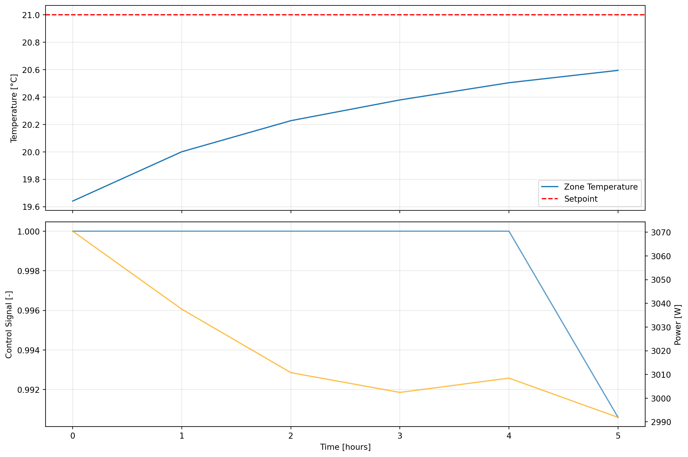
2. Compare KPIs across controllers:
# Run multiple controllers
controllers = {
    'Proportional': simple_proportional_controller,
    'MPC': mpc_controller_for_boptest,  # Your MPC implementation
}

comparison = {}
for name, controller in controllers.items():
    print(f"\nTesting {name} controller...")
    results = test_controller_on_boptest(url, testcase, controller)
    comparison[name] = results['kpis']

# Print comparison table
print("\n" + "="*70)
print(f"{'Controller':<20} {'Energy [kWh]':<15} {'Discomfort [Kh]':<15} {'Cost':<10}")
print("="*70)
for name, kpis in comparison.items():
    print(f"{name:<20} {kpis['ener_tot']:<15.2f} {kpis['tdis_tot']:<15.2f} {kpis['cost_tot']:<10.2f}")
3. Interpret KPI meanings:
ener_tot: Total energy consumption [kWh] - lower is bettertdis_tot: Thermal discomfort [Kh] - time-weighted temperature deviation outside comfort bounds (20-24°C) - lower is bettercost_tot: Operating cost based on time-of-use pricing - lower is betteremis_tot: CO₂ emissions - lower is better
Trade-offs to consider:
- Minimizing energy may increase discomfort
- Tight temperature control may increase energy use
- Cost depends on shifting loads to off-peak hours
- Best controller balances multiple objectives
11.6.6 Example: MPC Controller on BOPTEST
Now let’s adapt our MPC controller to work with BOPTEST. The key difference from our earlier example is that we need to:
- Work with BOPTEST’s actual building model (not our simple 1R1C approximation)
- Use BOPTEST’s forecast API to get weather predictions
- Return control inputs in BOPTEST format
Here’s a complete implementation:
import cvxpy as cp
import numpy as np
import requests

def mpc_controller_for_boptest(y, url, testid,
                                horizon=6,
                                T_set=273.15+21,
                                w_comfort=10.0,
                                w_energy=0.1):
    """
    MPC controller for BOPTEST using simplified 1R1C thermal model.

    Parameters
    ----------
    y : dict
        Current measurements from BOPTEST
    url : str
        BOPTEST service URL
    testid : str
        Test case ID
    horizon : int
        Prediction horizon [timesteps of 2 hours each]
    T_set : float
        Temperature setpoint [K]
    w_comfort : float
        Weight on comfort in cost function
    w_energy : float
        Weight on energy in cost function

    Returns
    -------
    u : dict
        Control inputs for BOPTEST
    """

    # Get current state
    T_current = y['reaTZon_y']  # Zone temperature [K]

    # Get weather forecast from BOPTEST
    try:
        forecast_response = requests.put(
            f'{url}/forecast/{testid}',
            json={
                'point_names': ['TDryBul'],
                'horizon': horizon * 3600,
                'interval': 3600
            }
        )
        if forecast_response.status_code == 200:
            forecast_data = forecast_response.json()['payload']
            T_amb_forecast = np.array(forecast_data['TDryBul'][:horizon])
        else:
            T_amb_forecast = np.full(horizon, 273.15 + 1.0)
    except:
        T_amb_forecast = np.full(horizon, 273.15 + 1.0)

    # Simplified building model parameters (approximation)
    # These would ideally be identified from BOPTEST data
    R = 0.002     # Thermal resistance [K/W]
    C = 2e7       # Thermal capacitance [J/K]
    dt = 3600     # Timestep [s] (1 hour)
    P_max_kW = 10.0  # Max heating power [kW]

    # Discrete model coefficients
    a = 1 - dt/(R*C)
    b = dt/C * 1000  # Multiplies kW, so scale by 1000
    e = dt/(R*C)

    # Define optimization variables
    T = cp.Variable(horizon + 1)
    u_kW = cp.Variable(horizon)

    # Constraints
    constraints = []
    constraints += [T[0] == T_current]  # Initial condition

    # Dynamics
    for k in range(horizon):
        constraints += [T[k+1] == a*T[k] + b*u_kW[k] + e*T_amb_forecast[k]]

    # Temperature bounds (comfort)
    T_min = 273.15 + 19  # 19°C (relaxed for feasibility)
    T_max = 273.15 + 24  # 24°C
    constraints += [T[1:] >= T_min]
    constraints += [T[1:] <= T_max]

    # Control bounds
    constraints += [u_kW >= 0]
    constraints += [u_kW <= P_max_kW]

    # Cost function
    comfort_cost = w_comfort * cp.sum_squares(T[:-1] - T_set)
    energy_cost = w_energy * cp.sum_squares(u_kW / P_max_kW)
    terminal_cost = w_comfort * cp.sum_squares(T[-1] - T_set)
    total_cost = comfort_cost + energy_cost + terminal_cost

    # Solve
    problem = cp.Problem(cp.Minimize(total_cost), constraints)
    try:
        problem.solve(verbose=False)

        if problem.status in ["optimal", "optimal_inaccurate"]:
            u_opt_kW = u_kW.value[0]  # Take first control action
            # Normalize to 0-1 range for BOPTEST
            u_normalized = float(np.clip(u_opt_kW / P_max_kW, 0.0, 1.0))
        else:
            # Fallback to proportional control
            error = max(0, T_set - T_current)
            u_normalized = min(2.0 * error, 1.0)
    except:
        # Fallback to proportional control
        error = max(0, T_set - T_current)
        u_normalized = min(2.0 * error, 1.0)

    # Return in BOPTEST format
    return {
        'oveHeaPumY_u': u_normalized,
        'oveHeaPumY_activate': 1
    }


# Run MPC controller on BOPTEST
url = 'http://13.217.71.86'
testcase = 'bestest_hydronic_heat_pump'

print("Testing MPC controller on BOPTEST...")
mpc_results = test_controller_on_boptest(
    url=url,
    testcase=testcase,
    controller=mpc_controller_for_boptest,
    simulation_days=0.25,
    step_size=3600  # 1 hour
)

print("\n" + "="*50)
print("MPC Controller Results:")
print("="*50)
print(f"Total Energy: {mpc_results['kpis']['ener_tot']:.2f} kWh")
print(f"Thermal Discomfort: {mpc_results['kpis']['tdis_tot']:.2f} Kh")
print(f"Operating Cost: {mpc_results['kpis']['cost_tot']:.2f} EUR")
print(f"CO2 Emissions: {mpc_results['kpis']['emis_tot']:.2f} kg")

# Plot results
import matplotlib.pyplot as plt

fig, (ax1, ax2) = plt.subplots(2, 1, figsize=(12, 8), sharex=True)

ax1.plot(mpc_results['time'], mpc_results['temperature'], label='Zone Temp', linewidth=2)
ax1.axhline(21, color='red', linestyle='--', label='Setpoint', alpha=0.7)
ax1.axhline(20, color='orange', linestyle=':', label='Comfort bounds', alpha=0.5)
ax1.axhline(24, color='orange', linestyle=':', alpha=0.5)
ax1.set_ylabel('Temperature [°C]')
ax1.legend()
ax1.grid(True, alpha=0.3)
ax1.set_title('MPC Controller on BOPTEST')

ax2.plot(mpc_results['time'], mpc_results['power']/1000, label='Heating Power',
         linewidth=2, color='green')
ax2.set_xlabel('Time [hours]')
ax2.set_ylabel('Power [kW]')
ax2.legend()
ax2.grid(True, alpha=0.3)

plt.tight_layout()
plt.show()
Testing MPC controller on BOPTEST...
Test ID: 4e62b15b-9e58-464e-bb82-f0f035ca75e8
Progress: 0/6 steps
==================================================
MPC Controller Results:
==================================================
Total Energy: 0.13 kWh
Thermal Discomfort: 7.02 Kh
Operating Cost: 0.03 EUR
CO2 Emissions: 0.02 kg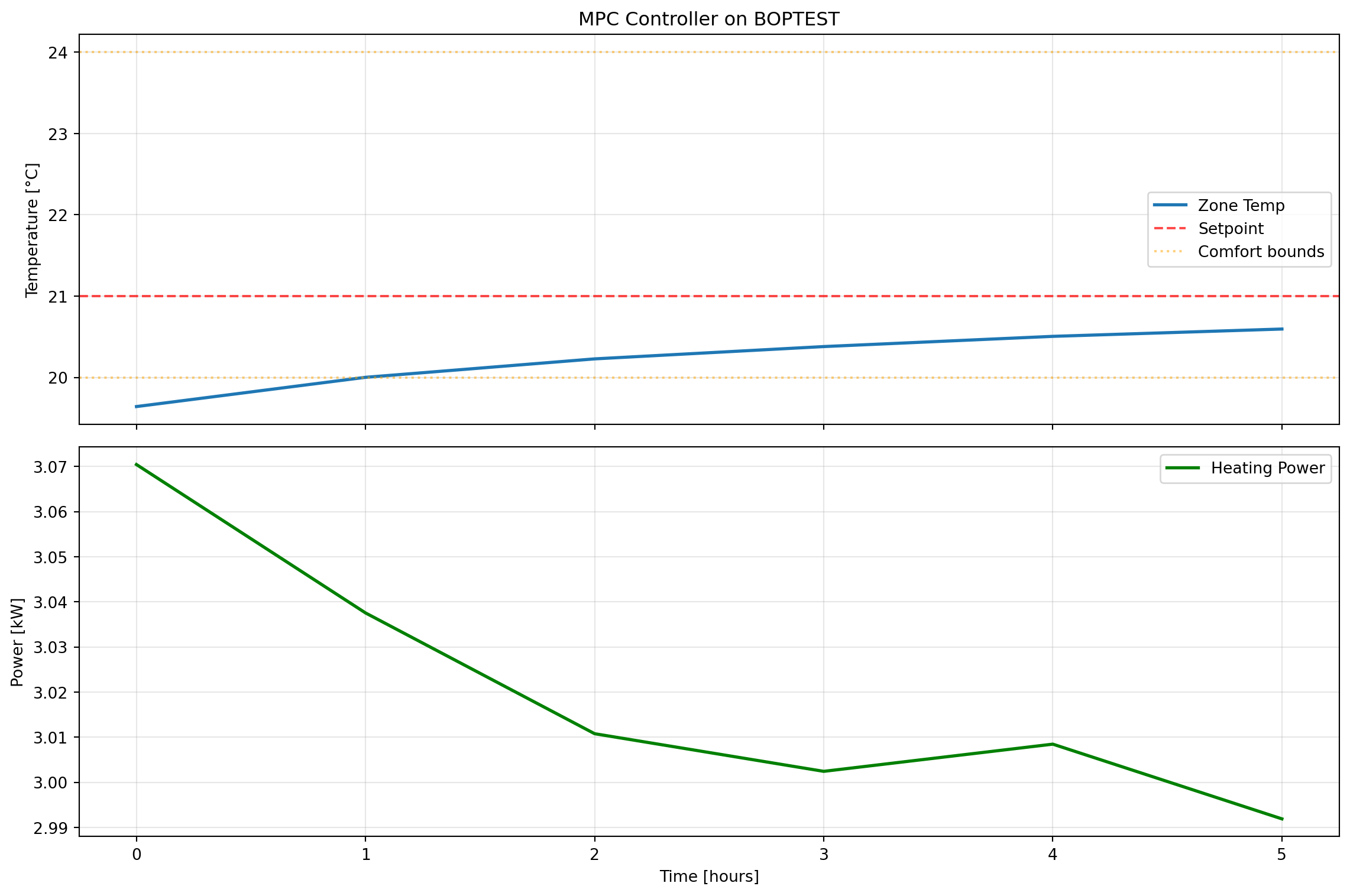
Key implementation notes:
Model mismatch: We use a simple 1R1C model even though BOPTEST has a more complex building. This is intentional - it demonstrates MPC’s robustness to model mismatch.
Forecast integration: The controller queries BOPTEST’s forecast API to get future weather predictions, which is crucial for MPC’s anticipatory behavior.
Fallback strategy: If the optimization fails, the controller falls back to simple proportional control. This ensures robustness.
Normalization: BOPTEST expects control signals in the 0-1 range, so we normalize the power output.
Error handling: The code includes try-except blocks to handle API failures gracefully.
11.7 Additional Resources
11.7.1 Key References
Blum, David, Javier Arroyo, Sen Huang, Jan Drgona, Filip Jorissen, Harald Taxt Walnum, Yan Chen, et al. “Building Optimization Testing Framework (BOPTEST) for Simulation-Based Benchmarking of Control Strategies in Buildings.” Journal of Building Performance Simulation 14, no. 5 (September 3, 2021): 586–610. https://doi.org/10.1080/19401493.2021.1986574
Drgoňa et al. “All you need to know about model predictive control for buildings” Annual Reviews in Control, Volume 50 (2020): 190-232. https://www.sciencedirect.com/science/article/pii/S1367578820300584
11.7.2 Software Tools
- cvxpy: https://www.cvxpy.org/
- BOPTEST: https://github.com/ibpsa/project1-boptest