10  Basics of AC Power Systems for Buildings

10.1 Lecture Overview

By the end of this module, students will be able to:

  • Understand how power is delivered from the grid to the electrical appliances/loads in a building, including:
    • The mathematical basis for AC power delivery:
      • Make use Ohm’s Law and Kirchhoff’s Voltage/Current Laws for DC circuits in order to derive an expression for power provided to an arbitrary RLC load
      • Distinguish between power losses and power transmitted in a circuit
      • Understand the steady-state and transient effects of the R, L, and C components for the load in the DC case
      • Recreate the expression for power under an AC voltage/current source and an arbitrary impedance
      • Recognize the steady-state and transient effects of the impedance (resistance + reactance) in the circuit for the AC case
      • Be able to use time domain (i.e., instantaneous) power expressions, as well as phasor and/or complex representations
    • The underlying physical mechanism from which sinusoidal voltage sources arise:
      • Understand the working principles and components of an AC electrical generator in general, and 3-phase generators in particular
      • Derive an expression for the voltage at each of the 3 phases of the generator (mathematically showing their phase difference)
      • Understand how power delivered/consumed and power generated need to be balanced, and the effect of this balance on the grid’s frequency
      • Describe, conceptually, how power from the generator gets transmitted to the distribution system and to the buildings in it
        • Understand the role of transformers in the transmission/distribution grids
        • Understand how split-phase systems to residential buildings in the US work
  • Analyze AC Power Usage
    • Starting from a known voltage source \(v(t)\) and current \(i(t)\), derive expressions for active, reactive, apparent and instantaneous power, as well as power factor
      • Understand the value of RMS and average quantities for voltage and current over some cycle-aligned period
      • Be able to leverage the phasor representation of these quantities
    • Calculate power quantities (active, reactive, etc.) from RMS or sub-cycle measurements of voltage and current
    • Be familiar with the VI trajectory (a single AC cycle plot of current versus voltage) as a visualization aid to differentiate between different load impedances
  • Review of DC Circuit Fundamentals
    • Ohm’s Law and Kirchhoff’s Laws
    • Power in DC circuits
    • RLC components and their behavior
  • Mathematical Framework for AC Power
    • Time domain representation
    • Phasor and complex notation
    • Impedance and reactance
  • AC Electrical Generators
    • Working principles and components
    • Single-phase and 3-phase generation
    • Grid frequency and power balance
  • Power Transmission and Distribution
    • Transformers and voltage levels
    • Split-phase residential systems
  • AC Power Analysis
    • Active, reactive, apparent, and instantaneous power
    • Power factor
    • RMS and average quantities
    • VI trajectory visualization

Understanding AC power systems is fundamental for the smart metering aspects of the final project. Students working on energy monitoring and analysis will need to apply concepts from this lecture to: - Interpret voltage and current measurements from smart meters - Calculate power consumption metrics - Understand load characteristics through VI trajectory analysis

10.2 Lecture Notes

10.2.1 Introduction: Why AC Power Matters for Buildings

Throughout this course, we’ve been building toward the goal of creating autonomous, sustainable buildings—spaces that can sense their environment, make intelligent decisions, and act to optimize energy consumption while maintaining occupant comfort. To achieve this vision, we need to understand not just thermal dynamics and comfort, but also how buildings consume and manage electrical energy.

Buildings account for approximately 40% of total energy consumption in developed countries, and addressing climate change will require deep decarbonization of this sector. A key strategy for decarbonization is electrification—transitioning away from fossil fuel combustion (natural gas furnaces, oil boilers) toward electric heat pumps, electric water heaters, and other high-efficiency electric technologies. This shift makes understanding electrical power systems in buildings more critical than ever for anyone working on building automation and energy management.

Today, nearly all electrical power delivered to buildings uses alternating current (AC) systems. AC power has dominated for over a century due to compelling advantages: transformers can efficiently step voltages up and down, enabling long-distance transmission at high voltages (minimizing resistive losses) and safe low-voltage distribution within buildings. The infrastructure—from power plants to distribution grids to building panels—is built around AC.

However, an interesting trend is emerging: DC (direct current) systems are making a comeback in buildings. Many modern loads (LED lighting, computers, electronics, variable-speed motor drives) internally convert AC to DC anyway, wasting energy in the conversion. Solar panels and batteries naturally produce and store DC power. Recent advances in DC-DC converters, solid-state transformers, and power electronics have made DC distribution systems increasingly viable. Some experts envision future buildings with DC microgrids, potentially offering higher efficiency and better integration with renewable energy and storage.

Despite this potential shift, AC power remains the foundation of building electrical systems today, and will for the foreseeable future. Understanding AC power is essential for:

  • Designing and analyzing smart metering systems (a focus of the final project)
  • Interpreting measurements from building energy management systems
  • Understanding how different loads behave and how to control them
  • Evaluating the energy and power quality impacts of building automation strategies

In this lecture, we’ll build a comprehensive understanding of AC power systems for buildings, starting from DC circuit fundamentals and progressing through AC circuit analysis, power generation and distribution, and practical measurement techniques.

10.2.2 Review of DC Circuit Fundamentals

Before diving into AC power, we’ll briefly review DC (direct current) circuit fundamentals. These concepts form the foundation for understanding AC circuits, and many of the analysis techniques carry over directly.

In DC circuits, voltage and current are constant over time (or vary slowly enough that we can treat them as constant). This simplification makes the mathematics more tractable and helps us build intuition that we’ll extend to the AC case.

Key Assumptions and Idealizations:

The circuit models we’ll use make several simplifying assumptions:

  1. Linearity: We assume that circuit elements obey linear relationships between voltage and current. For example, a resistor’s resistance doesn’t change with voltage or current. This is an approximation—real resistors heat up and change resistance—but it’s accurate enough for most practical purposes.

  2. Lumped elements: We treat resistors, inductors, and capacitors as discrete components with concentrated properties, ignoring distributed effects like the resistance of connecting wires or stray capacitance between traces.

  3. Ideal sources: We assume voltage and current sources can deliver arbitrary amounts of power without internal losses.

These assumptions enable us to use powerful analysis techniques like superposition (the response to multiple sources is the sum of individual responses) and allow us to build network models where complex systems are represented as interconnected components.

Connection to Thermal Systems:

If this sounds familiar, it should! In Lectures 5 and 6, we developed thermal network models for buildings using the exact same approach. We created lumped thermal resistances (R) and capacitances (C) to model heat flow and storage, then applied network analysis (analogous to Kirchhoff’s laws) to derive building thermal dynamics. The mathematical machinery is identical—only the physical interpretation changes:

Electrical Domain Thermal Domain
Voltage (\(V\)) Temperature (\(T\))
Current (\(I\)) Heat flow rate (\(\dot{Q}\))
Resistance (\(R\)) Thermal resistance (\(R_{th}\))
Capacitance (\(C\)) Thermal capacitance (\(C_{th}\))

This analogy is powerful and extends to mechanical systems as well (force ↔︎ voltage, velocity ↔︎ current). Once you understand the mathematical structure, you can apply it across multiple physical domains.

10.2.2.1 Ohm’s Law and Kirchhoff’s Laws

The fundamental laws governing circuit behavior are:

Ohm’s Law relates voltage across a resistor to the current through it: \[V = IR\]

where \(V\) is voltage (volts), \(I\) is current (amperes), and \(R\) is resistance (ohms, \(\Omega\)).

Kirchhoff’s Current Law (KCL) states that the sum of currents entering a node equals the sum leaving: \[\sum I_{in} = \sum I_{out}\]

This is just conservation of charge—electrons can’t accumulate at a node.

Kirchhoff’s Voltage Law (KVL) states that the sum of voltage drops around any closed loop is zero: \[\sum V_{loop} = 0\]

This follows from conservation of energy—no net energy is gained traveling around a closed path.

These laws apply to both DC and AC circuits, though in AC analysis we’ll extend them to work with complex quantities (phasors) rather than just real numbers.

10.2.2.2 Power in DC Circuits

Power is the rate of energy transfer or conversion. In electrical circuits, power delivered to a component is the product of voltage across it and current through it:

\[P = VI\]

where \(P\) is power in watts (W), \(V\) is voltage in volts (V), and \(I\) is current in amperes (A).

Derivation: Consider a charge \(\Delta q\) moving through a voltage difference \(V\). The energy transferred is \(\Delta E = V \Delta q\). The power is the rate of energy transfer: \[P = \frac{\Delta E}{\Delta t} = V \frac{\Delta q}{\Delta t} = VI\]

since current is defined as \(I = \Delta q / \Delta t\).

For a resistive load, we can substitute Ohm’s law (\(V = IR\)) to get alternative expressions:

\[P = VI = (IR)I = I^2 R\]

or equivalently,

\[P = VI = V \left(\frac{V}{R}\right) = \frac{V^2}{R}\]

These three equivalent forms are useful in different contexts:

  • \(P = VI\) when you know voltage and current
  • \(P = I^2R\) when you know current and resistance
  • \(P = V^2/R\) when you know voltage and resistance

In a resistor, electrical energy is converted to heat—the power \(P\) represents energy dissipation.

10.2.2.3 Resistors, Inductors, and Capacitors (RLC Components)

Electrical circuits are built from three fundamental passive elements: resistors (R), inductors (L), and capacitors (C). Each has a distinct voltage-current relationship and plays a different role in circuit behavior.

These elements have direct analogs in other physical systems, revealing the universal structure of dynamic systems:

Element Electrical Thermal Mechanical (Translational)
Dissipative Resistor (R) Thermal resistance Damper (friction)
Energy storage (type 1) Inductor (L) - Mass (inertia)
Energy storage (type 2) Capacitor (C) Thermal capacitance Spring (compliance)

The mathematical equations governing these elements are structurally identical across domains. This is why we could use RC circuit analysis techniques when modeling building thermal dynamics in earlier lectures.

10.2.2.3.1 Resistors

We’ve already introduced resistors through Ohm’s law (\(v = iR\)) and seen that they dissipate power as heat (\(p = i^2R = v^2/R\)).

What’s important to note about resistors is their instantaneous response: they have no memory or transient behavior. The current at any instant depends only on the voltage at that instant, not on past history. Whether in steady-state or during rapid changes, the relationship \(v = iR\) always holds immediately. Resistors dissipate energy continuously but do not store it.

10.2.2.3.2 Inductors

An inductor stores energy in a magnetic field created by current flowing through a coil of wire.

Voltage-current relationship: \[v = L \frac{di}{dt}\]

where \(L\) is the inductance in henries (H). The voltage across an inductor is proportional to the rate of change of current through it, not the current itself.

Energy storage: Energy is stored in the magnetic field: \[E = \frac{1}{2}LI^2\]

Unlike resistors, inductors don’t dissipate energy (in the ideal case)—they store it when current increases and release it when current decreases.

Transient behavior: Inductors oppose changes in current. If you try to suddenly change the current through an inductor, it produces a large opposing voltage. This creates time-dependent (transient) behavior. A key result: current through an inductor cannot change instantaneously. In steady-state DC conditions (where \(di/dt = 0\)), an inductor acts like a short circuit (zero voltage drop).

10.2.2.3.3 Capacitors

A capacitor stores energy in an electric field between two conductive plates separated by an insulator.

Voltage-current relationship: \[i = C \frac{dv}{dt}\]

where \(C\) is the capacitance in farads (F). The current through a capacitor is proportional to the rate of change of voltage across it.

Energy storage: Energy is stored in the electric field: \[E = \frac{1}{2}CV^2\]

Like inductors, ideal capacitors don’t dissipate energy—they store it when voltage increases and release it when voltage decreases.

Transient behavior: Capacitors oppose changes in voltage. If you try to suddenly change the voltage across a capacitor, it draws a large current. This creates time-dependent behavior. A key result: voltage across a capacitor cannot change instantaneously. In steady-state DC conditions (where \(dv/dt = 0\)), a capacitor acts like an open circuit (zero current flow).

10.2.2.4 Power Delivered to RLC Loads in DC Circuits

Now we can put these concepts together to understand power flow in circuits containing R, L, and C elements.

Recall that instantaneous power delivered to any circuit element is \(p(t) = v(t) \cdot i(t)\).

For a resistor: \[p_R(t) = v(t) \cdot i(t) = i^2(t) R\]

This power is dissipated as heat. The energy is permanently lost from the circuit.

For an inductor: \[p_L(t) = v(t) \cdot i(t) = L\frac{di}{dt} \cdot i = \frac{d}{dt}\left(\frac{1}{2}Li^2\right)\]

This power represents the rate of change of stored magnetic energy. When \(p_L > 0\), energy flows into the inductor (building up the magnetic field). When \(p_L < 0\), energy flows back out (as the field collapses). Over a complete cycle of charging and discharging, net energy dissipation is zero (in the ideal case).

For a capacitor: \[p_C(t) = v(t) \cdot i(t) = v \cdot C\frac{dv}{dt} = \frac{d}{dt}\left(\frac{1}{2}Cv^2\right)\]

Similarly, this represents the rate of change of stored electric energy. Energy sloshes in and out, but with no net dissipation over a complete cycle (again, ideally).

Key distinction:

  • Power losses (dissipated permanently): occur in resistive elements
  • Power transmitted (flowing back and forth): occurs in reactive elements (L and C) during energy storage and release

A note on idealizations: In real circuits, the wires connecting components also have resistance (line losses) and reactance (line impedance—small amounts of inductance and capacitance). Power is dissipated in these wires, and they affect circuit dynamics. However, for our analysis, we’ll assume these effects are negligible compared to the actual circuit components. This is reasonable for short wire runs and moderate currents, but in long-distance power transmission or high-current applications, line losses and reactance become very important.

This distinction between dissipated power and transmitted power becomes crucial when we move to AC circuits, where we’ll formalize these concepts as real power (dissipated in R) versus reactive power (oscillating in L and C).

10.2.3 Transition to AC: Why Alternating Current?

Now that we understand DC circuits, why complicate things by making voltage and current vary sinusoidally over time? The answer lies in the practical challenges of power distribution.

Historical Context: The War of Currents

In the late 1800s, Thomas Edison championed direct current for electrical distribution, building DC power systems across major cities. Nikola Tesla and George Westinghouse advocated for alternating current. This “War of Currents” was ultimately won by AC, not because AC is inherently superior for all applications, but because of one critical advantage: transformers.

The Transformer Advantage

Transformers can efficiently change AC voltage levels using electromagnetic induction—the same principle behind inductors. This capability is crucial for power distribution:

  1. High-voltage transmission reduces line losses: Recall that power loss in a wire is \(P_{loss} = I^2 R_{line}\). For a given amount of power \(P = VI\) to transmit, we can use high voltage and low current, dramatically reducing resistive losses in transmission lines. AC systems routinely transmit at hundreds of kilovolts, then step down to safe levels for buildings.

  2. Transformers are simple and efficient: With no moving parts, transformers can convert voltage levels at 95-99% efficiency. Early DC systems had no equivalent technology—Edison’s plants had to be located within about a mile of customers due to unacceptable line losses at the low DC voltages used.

  3. Safety and versatility: AC systems generate at optimal voltages for generators, transmit at high voltages for efficiency, and deliver at safe voltages (120V/240V) for end users, all using transformers.

What Has Changed Since Then?

The War of Currents was decided by the technology available in the 1890s. Today, power electronics have changed the landscape:

  • Modern DC-DC converters (based on high-frequency switching) can now change DC voltage levels efficiently, something impossible in Edison’s era
  • High-voltage DC (HVDC) transmission is now used for very long distances and undersea cables, where AC’s reactive losses become problematic
  • Solar panels, batteries, and LED lighting all operate on DC internally
  • Modern electronics (computers, phone chargers, variable-speed drives) convert AC to DC immediately upon receiving power, wasting energy in the conversion

Despite these developments, AC remains dominant because of massive infrastructure investment and the fact that transformers are still simpler and cheaper than power electronics for most applications. However, DC microgrids within buildings and DC distribution systems are gaining traction, especially where solar and battery storage are involved.

For the foreseeable future, you’ll need to understand both: AC for the grid and building mains, DC for electronics and emerging distributed energy systems.

10.2.4 Mathematical Framework for AC Power

In DC circuits, voltage and current are constant, making analysis straightforward. In AC circuits, voltage and current vary sinusoidally with time, which fundamentally changes the circuit dynamics. This time-dependence means that inductors and capacitors—which were relatively simple in DC steady-state—now play active roles, continuously storing and releasing energy.

To analyze AC circuits, we need mathematical tools that handle these time-varying quantities efficiently. We’ll develop three representations: time domain (using trigonometric functions), phasor domain (using rotating vectors), and complex notation (using complex numbers). Each has its advantages depending on what we’re trying to calculate.

10.2.4.1 Sinusoidal Voltage and Current Sources

AC power systems use sinusoidal voltage and current waveforms—signals that vary as sine or cosine functions of time. A sinusoidal voltage can be written as:

\[v(t) = V_m \sin(\omega t + \phi)\]

where:

  • \(V_m\) is the amplitude (peak voltage) in volts
  • \(\omega\) is the angular frequency in radians per second
  • \(\phi\) is the phase angle in radians (or degrees), which determines where the waveform starts at \(t = 0\)

The frequency \(f\) (in Hertz, cycles per second) relates to angular frequency by: \[\omega = 2\pi f\]

In the US, the grid operates at \(f = 60\) Hz, so \(\omega = 2\pi \cdot 60 \approx 377\) rad/s. In most other countries, \(f = 50\) Hz.

Why sinusoids? Real AC sources aren’t perfectly sinusoidal—they have some distortion. However, if we assume our circuits are linear, then the superposition principle applies: the circuit’s response to a sum of inputs equals the sum of responses to individual inputs. This means we can decompose any periodic waveform into a sum of sinusoids at different frequencies (Fourier series), analyze the circuit’s response to each sinusoid separately, and add up the results. For power system analysis, the fundamental frequency (60 Hz) typically dominates, so we often analyze only that component.

10.2.4.2 Time Domain Representation

In the time domain, we explicitly write voltage and current as functions of time. For an AC circuit with sinusoidal excitation:

Voltage: \[v(t) = V_m \sin(\omega t + \phi_v)\]

Current: \[i(t) = I_m \sin(\omega t + \phi_i)\]

The phase angles \(\phi_v\) and \(\phi_i\) are generally different (i.e., in AC circuits, voltage and current don’t necessarily reach their peaks at the same time). Why? Well, if the current drawn was all for power being dissipated through resistive loads, then they would be the same. But as we saw before, inductors and capacitors store energy in magnetic and electric fields, thus causing a misalignment between the current and voltage sinusoids. Thus, the phase difference \(\phi = \phi_v - \phi_i\) is crucial for understanding power flow.

Let’s visualize this with an example where voltage and current are out of phase:

Code
import numpy as np
import matplotlib.pyplot as plt

# Parameters
f = 60  # Hz (US grid frequency)
omega = 2 * np.pi * f  # Angular frequency
V_m = 170  # Peak voltage (about 120 V RMS)
I_m = 100   # Peak current
phi_v = 0  # Voltage phase angle (reference)
phi_i = -np.pi/4  # Current lags voltage by 45 degrees

# Time vector (3 cycles)
t = np.linspace(0, 3/f, 1000)

# Calculate waveforms
v = V_m * np.sin(omega * t + phi_v)
i = I_m * np.sin(omega * t + phi_i)

# Plot
plt.figure(figsize=(8, 4))
plt.plot(t * 1000, v, label='Voltage $v(t)$', linewidth=2)
plt.plot(t * 1000, i, label='Current $i(t)$', linewidth=2)
plt.xlabel('Time (ms)')
plt.ylabel('Amplitude')
plt.title('AC Voltage and Current (60 Hz, current lagging by 45°)')
plt.grid(True, alpha=0.3)
plt.legend()
plt.axhline(y=0, color='k', linewidth=0.5)
plt.tight_layout()
plt.show()
Figure 10.1: Voltage and current waveforms in an AC circuit with phase difference

Notice that the current waveform reaches its peak after the voltage waveform—we say the current lags the voltage. This happens when the load contains inductance (like motors or transformers). Conversely, capacitive loads cause current to lead voltage.

10.2.4.3 Impedance and Reactance

In DC circuits, Ohm’s law states that \(V = IR\), where resistance \(R\) relates voltage to current. In AC circuits, we need a generalization that accounts for the phase difference between voltage and current.

Impedance (\(Z\)) is the AC generalization of resistance. It relates the phasor representations of voltage and current:

\[\tilde{V} = \tilde{Z} \cdot \tilde{I}\]

where the tilde (\(\tilde{}\)) denotes phasor quantities (we’ll define phasors formally in the next section).

Impedance is a complex number with both magnitude and phase:

\[Z = R + jX\]

where:

  • \(R\) is the resistance (real part), representing energy dissipation
  • \(X\) is the reactance (imaginary part), representing energy storage
  • \(j = \sqrt{-1}\) is the imaginary unit

The magnitude \(|Z| = \sqrt{R^2 + X^2}\) determines how much the impedance opposes current flow. The phase angle \(\theta = \arctan(X/R)\) determines the phase shift between voltage and current.

Reactance comes in two flavors:

  • Inductive reactance (\(X_L > 0\)): Causes current to lag voltage. Associated with magnetic energy storage in inductors.
  • Capacitive reactance (\(X_C < 0\)): Causes current to lead voltage. Associated with electric energy storage in capacitors.
10.2.4.3.1 Impedance of R, L, and C in AC Circuits

Let’s derive the impedance of each fundamental circuit element:

Resistor: \[Z_R = R\]

For a resistor, voltage and current are always in phase. The impedance is purely real with no reactive component. The resistor behaves the same in AC as in DC (at any instant, \(v = iR\)).

Inductor: \[Z_L = j\omega L\]

Recall that for an inductor, \(v = L \frac{di}{dt}\). When current is sinusoidal, \(i(t) = I_m \sin(\omega t)\), the voltage becomes: \[v(t) = L\frac{d}{dt}[I_m \sin(\omega t)] = \omega L I_m \cos(\omega t) = \omega L I_m \sin(\omega t + 90°)\]

The voltage leads the current by 90°. The magnitude ratio is \(\omega L\), which we call the inductive reactance: \(X_L = \omega L\). In complex notation, this 90° lead is represented by multiplication by \(j\), giving \(Z_L = j\omega L\).

Physical interpretation: Higher frequency (\(\omega\)) or larger inductance (\(L\)) creates more opposition to current changes, increasing reactance.

Capacitor: \[Z_C = \frac{1}{j\omega C} = -\frac{j}{\omega C}\]

For a capacitor, \(i = C \frac{dv}{dt}\). When voltage is sinusoidal, \(v(t) = V_m \sin(\omega t)\), the current becomes: \[i(t) = C\frac{d}{dt}[V_m \sin(\omega t)] = \omega C V_m \cos(\omega t) = \omega C V_m \sin(\omega t + 90°)\]

The current leads the voltage by 90°. Equivalently, voltage lags current by 90°. The magnitude ratio is \(\frac{1}{\omega C}\), which we call the capacitive reactance: \(X_C = -\frac{1}{\omega C}\). In complex notation, this 90° lag is represented by division by \(j\) (or multiplication by \(-j\)), giving \(Z_C = \frac{1}{j\omega C}\).

Physical interpretation: Higher frequency (\(\omega\)) or larger capacitance (\(C\)) allows more current to flow, decreasing the magnitude of impedance.

10.2.4.4 Phasor Representation

Earlier, we mentioned that phasor representation is one of three mathematical tools for AC circuit analysis. Now let’s dive into what phasors actually are and why they’re so powerful.

Working with sinusoidal functions directly in the time domain involves messy trigonometric identities and differential equations. Phasors provide an elegant shortcut that converts these differential equations into simple algebra.

Formal definition:

A phasor is a complex number that represents the amplitude and phase of a sinusoidal signal, with the implicit understanding that the signal oscillates at a known frequency \(\omega\).

For a sinusoidal voltage: \[v(t) = V_m \sin(\omega t + \phi)\]

The corresponding phasor is: \[\tilde{V} = V_m e^{j\phi} = V_m \angle \phi\]

The phasor captures two pieces of information:

  • Magnitude: \(|\tilde{V}| = V_m\) (the amplitude)
  • Phase angle: \(\angle \tilde{V} = \phi\) (the phase at \(t=0\))

The notation \(V_m \angle \phi\) is called polar form. We can also write it in rectangular form as \(\tilde{V} = V_m \cos\phi + j V_m \sin\phi\).

Key insight: In steady-state AC analysis, all voltages and currents oscillate at the same frequency \(\omega\). The phasor representation “factors out” the common \(e^{j\omega t}\) term, leaving only the magnitude and relative phase. This dramatically simplifies analysis.

From Time Domain to Phasor Domain

The magic of phasors is that differentiation in the time domain becomes multiplication by \(j\omega\) in the phasor domain.

If \(v(t) = V_m \sin(\omega t + \phi)\), then: \[\frac{dv}{dt} = \omega V_m \cos(\omega t + \phi) = \omega V_m \sin(\omega t + \phi + 90°)\]

In phasor notation, this becomes simply: \[\frac{d\tilde{V}}{dt} \longleftrightarrow j\omega \tilde{V}\]

The 90° phase shift (from differentiation) is captured by multiplying by \(j\) (which rotates a complex number by 90°), and the amplitude scaling by \(\omega\) appears naturally.

This is why the impedances we derived earlier have the form they do:

  • Inductor: \(v = L\frac{di}{dt}\) becomes \(\tilde{V} = j\omega L \tilde{I}\), so \(Z_L = j\omega L\)
  • Capacitor: \(i = C\frac{dv}{dt}\) becomes \(\tilde{I} = j\omega C \tilde{V}\), so \(Z_C = \frac{1}{j\omega C}\)

Visualizing Phasors

Phasors can be visualized as rotating vectors in the complex plane:

Figure 10.2: Phasor representation: the phasor (left) encodes amplitude and phase angle, which determines the shift of the full sinusoid in the time domain (right)

The phasor captures the amplitude \(V_m\) and phase angle \(\phi\) of a sinusoidal signal. In the time domain, a nonzero phase angle \(\phi\) shifts the entire sinusoid earlier (for \(\phi > 0\), a “lead”) or later (for \(\phi < 0\), a “lag”) relative to the reference signal \(V_m \sin(\omega t)\).

Using Phasors in Circuit Analysis

With phasors, circuit analysis becomes algebraic:

  • Ohm’s law: \(\tilde{V} = \tilde{Z} \cdot \tilde{I}\) (complex multiplication)
  • KCL: \(\sum \tilde{I}_{in} = \sum \tilde{I}_{out}\) (complex addition)
  • KVL: \(\sum \tilde{V}_{loop} = 0\) (complex addition)

No differential equations required! We solve for phasor voltages and currents, then convert back to time domain if needed.

10.2.4.5 Complex Representation of AC Quantities

The phasor concept rests on a mathematical foundation: Euler’s formula, which connects complex exponentials to trigonometric functions.

Euler’s Formula: \[e^{j\theta} = \cos\theta + j\sin\theta\]

This identity allows us to represent sinusoidal functions as the real (or imaginary) part of complex exponentials.

Representing Sinusoids with Complex Exponentials

A sinusoidal voltage \(v(t) = V_m \sin(\omega t + \phi)\) can be written as: \[v(t) = \text{Im}\{V_m e^{j(\omega t + \phi)}\}\]

or equivalently (using \(\sin = -\text{Im}\{e^{j\cdot}\}\) or appropriate phase shifts): \[v(t) = \text{Re}\{V_m e^{j(\omega t + \phi + 90°)}\}\]

We can factor this as: \[v(t) = \text{Im}\{V_m e^{j\phi} \cdot e^{j\omega t}\} = \text{Im}\{\tilde{V} e^{j\omega t}\}\]

where \(\tilde{V} = V_m e^{j\phi}\) is the phasor we defined earlier!

The Power of Complex Representation

The key insight: when all signals oscillate at the same frequency \(\omega\), they all share the common factor \(e^{j\omega t}\). We can:

  1. Factor out the \(e^{j\omega t}\) term
  2. Work with just the complex amplitudes (phasors) \(\tilde{V}, \tilde{I}, \tilde{Z}\)
  3. Factor back in the \(e^{j\omega t}\) and take the real/imaginary part to get the time-domain result

This transforms differential equations into algebraic equations with complex numbers.

Complex Number Arithmetic

Complex numbers can be expressed in two forms:

Rectangular (Cartesian) form: \[Z = a + jb\] where \(a\) is the real part and \(b\) is the imaginary part.

Polar (magnitude-angle) form: \[Z = r e^{j\theta} = r \angle \theta\] where \(r = |Z| = \sqrt{a^2 + b^2}\) is the magnitude and \(\theta = \arctan(b/a)\) is the phase angle.

Conversion between forms:

  • Rectangular to polar: \(r = \sqrt{a^2 + b^2}\), \(\theta = \arctan(b/a)\)
  • Polar to rectangular: \(a = r\cos\theta\), \(b = r\sin\theta\)

Operations:

  • Addition/subtraction: Use rectangular form \[(a_1 + jb_1) + (a_2 + jb_2) = (a_1 + a_2) + j(b_1 + b_2)\]

  • Multiplication/division: Use polar form \[r_1\angle\theta_1 \times r_2\angle\theta_2 = (r_1 r_2) \angle (\theta_1 + \theta_2)\] \[\frac{r_1\angle\theta_1}{r_2\angle\theta_2} = \frac{r_1}{r_2} \angle (\theta_1 - \theta_2)\]

Consider a series RL circuit with \(R = 10\,\Omega\), \(L = 20\) mH at \(f = 60\) Hz.

The total impedance is: \[Z_{total} = R + Z_L = R + j\omega L\]

With \(\omega = 2\pi \cdot 60 \approx 377\) rad/s: \[Z_{total} = 10 + j(377)(0.02) = 10 + j7.54\,\Omega\]

In polar form: \[|Z_{total}| = \sqrt{10^2 + 7.54^2} = 12.53\,\Omega\] \[\angle Z_{total} = \arctan(7.54/10) = 37.0°\]

So \(Z_{total} = 12.53\angle 37.0°\,\Omega\).

If we apply a voltage \(\tilde{V} = 120\angle 0°\) V, the current is: \[\tilde{I} = \frac{\tilde{V}}{Z_{total}} = \frac{120\angle 0°}{12.53\angle 37.0°} = 9.58\angle -37.0°\,\text{A}\]

The \(-37.0°\) phase means current lags voltage by 37°, which makes sense for an inductive load.

10.2.5 Instantaneous Power in AC Circuits

In DC circuits, power is simply \(P = VI\), constant over time. In AC circuits, voltage and current vary sinusoidally, so instantaneous power \(p(t) = v(t) \cdot i(t)\) also varies with time. Understanding this time variation is crucial for comprehending how energy flows in AC systems.

Why instantaneous power matters:

  • It reveals the dynamic energy exchange between source and load
  • It explains why some power “sloshes back and forth” without being consumed
  • It’s the foundation for defining active (real) vs. reactive power
  • Smart meters measure instantaneous power to calculate energy consumption

Let’s visualize how instantaneous power behaves:

Figure 10.3: Voltage, current, and instantaneous power for an inductive load

Notice that:

  1. Power oscillates at twice the line frequency (120 Hz for 60 Hz AC)
  2. Power can be negative (energy flowing back from load to source)
  3. The average power is positive (net energy flows to the load)

10.2.5.1 Derivation from Time Domain Expressions

Let’s derive the mathematical expression for instantaneous power.

Given: \[v(t) = V_m \sin(\omega t)\] \[i(t) = I_m \sin(\omega t - \phi)\]

where \(\phi\) is the phase difference (current lags voltage by \(\phi\) for inductive loads).

The instantaneous power is: \[p(t) = v(t) \cdot i(t) = V_m \sin(\omega t) \cdot I_m \sin(\omega t - \phi)\]

Using the trigonometric identity: \[\sin A \sin B = \frac{1}{2}[\cos(A - B) - \cos(A + B)]\]

We get: \[p(t) = V_m I_m \sin(\omega t) \sin(\omega t - \phi)\] \[= \frac{V_m I_m}{2}[\cos(\phi) - \cos(2\omega t - \phi)]\]

Rearranging: \[p(t) = \frac{V_m I_m}{2}\cos(\phi) - \frac{V_m I_m}{2}\cos(2\omega t - \phi)\]

This can be written as: \[\boxed{p(t) = P_{avg} + P_{osc}\cos(2\omega t - \phi)}\]

where:

  • \(P_{avg} = \frac{V_m I_m}{2}\cos(\phi)\) is the average power (DC component)
  • \(P_{osc} = \frac{V_m I_m}{2}\) is the amplitude of oscillation (AC component at \(2\omega\))

Notice that, of these two, only \(P_{osc}\) has a time (\(t\)) component.

Expressing instantaneous power in terms of RMS quantities:

Since for sinusoidal waveforms \(V_{rms} = \frac{V_m}{\sqrt{2}}\) and \(I_{rms} = \frac{I_m}{\sqrt{2}}\), the product \(\frac{V_m I_m}{2}\) is simply \(V_{rms} I_{rms}\). This lets us rewrite the instantaneous power as:

\[p(t) = V_{rms} I_{rms} \cos(\phi) - V_{rms} I_{rms} \cos(2\omega t - \phi)\]

This form is convenient because RMS values are what meters display and what equipment is rated for. It also makes the connection to the power quantities we define next (active, reactive, apparent) more direct, since those are all expressed in terms of RMS values.

The RMS (root-mean-square) value of a periodic signal \(x(t)\) with period \(T\) is defined as:

\[x_{rms} = \sqrt{\frac{1}{T}\int_0^T x^2(t) \, dt}\]

For a sinusoidal voltage \(v(t) = V_m \sin(\omega t)\), we compute each step:

1. Square: \[v^2(t) = V_m^2 \sin^2(\omega t)\]

2. Mean (average over one period):

Using the trigonometric identity \(\sin^2(\theta) = \frac{1 - \cos(2\theta)}{2}\):

\[\frac{1}{T}\int_0^T V_m^2 \sin^2(\omega t) \, dt = \frac{V_m^2}{T}\int_0^T \frac{1 - \cos(2\omega t)}{2} \, dt\]

\[= \frac{V_m^2}{2T}\left[\int_0^T 1 \, dt - \int_0^T \cos(2\omega t) \, dt\right]\]

The first integral evaluates to \(T\). The second integral evaluates to zero because \(\cos(2\omega t)\) completes exactly two full cycles over one period \(T = \frac{2\pi}{\omega}\), and the positive and negative areas cancel. Therefore:

\[\frac{1}{T}\int_0^T v^2(t) \, dt = \frac{V_m^2}{2}\]

3. Root: \[V_{rms} = \sqrt{\frac{V_m^2}{2}} = \frac{V_m}{\sqrt{2}}\]

The same result applies to current: \(I_{rms} = \frac{I_m}{\sqrt{2}}\). Multiplying:

\[V_{rms} \cdot I_{rms} = \frac{V_m}{\sqrt{2}} \cdot \frac{I_m}{\sqrt{2}} = \frac{V_m I_m}{2}\]

which is exactly the factor that appears in our instantaneous power expression.

10.2.5.2 Power Oscillation at Twice the Line Frequency

Why does power oscillate at \(2\omega\)?

Each voltage and current cycle contains both positive and negative half-cycles. When we multiply them:

  • Positive voltage × positive current = positive power
  • Negative voltage × negative current = positive power (two negatives!)
  • Positive voltage × negative current = negative power
  • Negative voltage × positive current = negative power

This pattern repeats twice per AC cycle, hence the \(2\omega\) frequency.

Physical interpretation:

  1. When \(p(t) > 0\): Energy flows from source to load (load absorbs energy)
  2. When \(p(t) < 0\): Energy flows from load back to source (load returns stored energy)
  3. Average over a cycle: Net energy transfer equals \(P_{avg} = \frac{V_m I_m}{2}\cos(\phi)\)

Key observations:

  • If \(\phi = 0\) (resistive load): \(P_{avg}\) is maximum, power never goes negative, all energy is dissipated
  • If \(\phi = 90°\) (purely reactive load): \(P_{avg} = 0\), power oscillates symmetrically around zero, no net energy transfer—energy just sloshes back and forth
  • If \(0 < \phi < 90°\) (typical load): Some energy is dissipated, some oscillates

The oscillating component represents reactive power—energy that’s temporarily stored in inductors and capacitors, then returned to the source. Notice too that \(P_{osc}\), though time-varying, behaves as a sinusoid which means that over a cycle it has the same amount of positive and negative contributions (i.e., it averages to zero over integer number of cycles).

10.2.6 Active, Reactive, and Apparent Power

Again, the instantaneous power derivation revealed that AC power has two components: a DC (average) component and an oscillating component. This leads us to define three distinct power quantities that characterize AC systems: active power, reactive power, and apparent power.

These three quantities are fundamental to understanding AC power systems, utility billing, and equipment sizing.

10.2.6.1 Active Power (Real Power)

Active power (also called real power) is the average power delivered to the load over a complete cycle. This is the power that actually does useful work—it’s converted to heat, light, mechanical work, etc.

Definition: \[P = V_{rms} I_{rms} \cos(\phi)\]

where:

  • \(V_{rms}\) is the RMS voltage
  • \(I_{rms}\) is the RMS current
  • \(\phi\) is the phase angle between voltage and current
  • \(\cos(\phi)\) is the power factor

Units: Watts (W)

Physical meaning: Active power represents the net energy transfer per unit time from source to load. It’s what you pay for on your electric bill (measured in kWh = kilowatt-hours).

From our earlier derivation: We showed that average power is \(P_{avg} = \frac{V_m I_m}{2}\cos(\phi)\). Since \(V_{rms} = \frac{V_m}{\sqrt{2}}\) and \(I_{rms} = \frac{I_m}{\sqrt{2}}\), we have: \[P = V_{rms} I_{rms} \cos(\phi)\]

Special cases:

  • Resistive load (\(\phi = 0°\)): \(P = V_{rms} I_{rms}\) (maximum power transfer)
  • Purely reactive load (\(\phi = 90°\)): \(P = 0\) (no net energy transfer)

10.2.6.2 Reactive Power

Reactive power represents the power that oscillates between source and load without being consumed. It’s associated with energy storage in inductors and capacitors.

Definition: \[Q = V_{rms} I_{rms} \sin(\phi)\]

Units: Volt-Amperes Reactive (VAR)

Physical meaning: Reactive power doesn’t do useful work, but it’s necessary for:

  • Creating magnetic fields in motors and transformers
  • Creating electric fields in capacitors
  • Maintaining voltage levels in the power system

Sign convention:

  • \(Q > 0\) (positive): Inductive reactive power (current lags voltage, typical for motors, transformers)
  • \(Q < 0\) (negative): Capacitive reactive power (current leads voltage, typical for capacitor banks)

Why it matters: Although reactive power doesn’t do work, it requires current to flow in transmission lines, causing resistive losses (\(I^2 R\)). Utilities often charge industrial customers for excessive reactive power.

10.2.6.3 Apparent Power

Apparent power is the product of RMS voltage and RMS current, without considering the phase angle.

Definition: \[S = V_{rms} I_{rms}\]

Units: Volt-Amperes (VA)

Physical meaning: Apparent power represents the total power that must be supplied by the source and carried by the wires, regardless of how much actually does useful work. It determines:

  • Wire sizing (current carrying capacity)
  • Generator/transformer ratings
  • Circuit breaker ratings

Equipment is rated in VA (or kVA, MVA) rather than watts because it must handle the total current, not just the portion doing useful work.

10.2.6.4 Power Triangle

The relationship between active, reactive, and apparent power can be visualized geometrically as a power triangle:

Figure 10.4: Power triangle showing relationship between P, Q, and S

Mathematical relationships: \[S^2 = P^2 + Q^2\] \[P = S \cos(\phi)\] \[Q = S \sin(\phi)\] \[\phi = \arctan(Q/P)\]

The power triangle is analogous to the impedance triangle (\(Z = R + jX\)), which is why we use complex notation for power calculations.

10.2.6.5 Power Factor

Power factor (PF) is the ratio of active power to apparent power:

\[\text{PF} = \frac{P}{S} = \cos(\phi)\]

Range: \(0 \leq \text{PF} \leq 1\)

Interpretation:

  • PF = 1 (unity power factor): Ideal case, all power is active (resistive load)
  • PF = 0: Worst case, all power is reactive (purely reactive load)
  • PF = 0.7-0.9: Typical for industrial loads (motors, fluorescent lighting)

Why power factor matters:

  1. Utility billing: Many utilities charge penalties for low power factor (typically below 0.9) because it forces them to generate and transmit more current for the same useful power

  2. System efficiency: Low power factor means:

    • Higher current for same active power → higher \(I^2R\) losses in wires
    • Larger generators, transformers, and wiring needed
    • Reduced system capacity
  3. Power factor correction: Capacitor banks are often installed to cancel inductive reactive power, improving power factor

Example: A motor drawing 10 A at 120 V with PF = 0.8:

  • Apparent power: \(S = 120 \times 10 = 1200\) VA
  • Active power: \(P = 1200 \times 0.8 = 960\) W (what you pay for)
  • Reactive power: \(Q = \sqrt{1200^2 - 960^2} = 720\) VAR (wasted current)

Leading vs. Lagging:

  • Lagging power factor (\(Q > 0\)): Current lags voltage (inductive load) - most common
  • Leading power factor (\(Q < 0\)): Current leads voltage (capacitive load) - less common
  • By convention, we often specify PF as “0.8 lagging” or “0.9 leading”

10.2.7 AC Electrical Generators: The Source of Sinusoidal Voltage

We’ve been working with sinusoidal voltage sources throughout this lecture, treating them as given. But where do these sinusoidal waveforms actually come from? The answer lies in electromagnetic induction and the design of AC generators (also called alternators).

Understanding generator operation helps explain:

  • Why AC power is naturally sinusoidal
  • The relationship between mechanical rotation speed and electrical frequency
  • How the grid’s frequency is maintained
  • Why three-phase power is used for generation and transmission

10.2.7.1 Basic Principles of Electromagnetic Induction

The fundamental principle behind all electrical generators is Faraday’s Law of Electromagnetic Induction:

\[\mathcal{E} = -\frac{d\Phi_B}{dt}\]

where:

  • \(\mathcal{E}\) is the induced electromotive force (EMF), or voltage
  • \(\Phi_B\) is the magnetic flux through a conductor
  • The negative sign indicates the direction (Lenz’s law)

In plain language: When the magnetic flux through a conductor changes, a voltage is induced in that conductor.

How generators use this principle:

  1. Create a strong magnetic field (using permanent magnets or electromagnets)
  2. Rotate a conductor (coil of wire) through this magnetic field
  3. As the coil rotates, the magnetic flux through it changes continuously
  4. This changing flux induces a voltage in the coil

Why the output is sinusoidal:

When a coil rotates at constant angular velocity \(\omega\) in a uniform magnetic field, the flux through it varies as: \[\Phi_B(t) = \Phi_{max} \cos(\omega t)\]

Taking the derivative: \[\mathcal{E}(t) = -\frac{d}{dt}[\Phi_{max} \cos(\omega t)] = \omega \Phi_{max} \sin(\omega t)\]

The induced voltage is naturally sinusoidal. The mechanical rotation creates an electrical sine wave.

10.2.7.2 Components of an AC Generator

An AC generator consists of these main parts:

1. Stator (stationary part):

  • The outer shell with coils of wire (windings) where voltage is induced
  • In large generators, this is the component that outputs electrical power
  • Made of laminated steel to reduce eddy current losses

2. Rotor (rotating part):

  • The spinning component that creates the rotating magnetic field
  • Contains electromagnets (field windings) powered by DC current
  • Mechanically coupled to a turbine (steam, hydro, wind, etc.)

3. Field windings:

  • Coils on the rotor that create the magnetic field
  • Powered by DC current through slip rings or a separate exciter
  • The strength of this field determines the output voltage magnitude

4. Armature windings:

  • Coils in the stator where AC voltage is induced
  • Connected to the output terminals
  • Typically three separate sets of windings for three-phase output

5. Mechanical drive system:

  • Steam turbine (coal, nuclear, natural gas plants)
  • Hydro turbine (hydroelectric dams)
  • Wind turbine (wind farms)
  • Diesel/gas engine (backup generators)

6. Voltage regulator:

  • Controls the DC current to the field windings
  • Adjusts output voltage to maintain desired level (e.g., 13.8 kV)

10.2.7.3 Single-Phase Generator Operation

Let’s trace how mechanical rotation creates electrical voltage in the simplest case: a single-phase generator.

Setup: A rectangular coil with \(N\) turns rotates in a uniform magnetic field \(B\) at angular velocity \(\omega\).

The rotating coil:

  • As the coil rotates, the angle \(\theta = \omega t\) between the coil’s normal and the magnetic field changes
  • The magnetic flux through the coil is: \(\Phi_B = NBA\cos(\omega t)\) where \(A\) is the coil area

Induced voltage (from Faraday’s law): \[v(t) = -N\frac{d\Phi_B}{dt} = NBA\omega \sin(\omega t) = V_m \sin(\omega t)\]

where \(V_m = NBA\omega\) is the peak voltage.

Key insights:

  • The amplitude \(V_m\) depends on: magnetic field strength (\(B\)), number of turns (\(N\)), coil area (\(A\)), and rotation speed (\(\omega\))
  • The frequency is \(f = \omega/(2\pi)\), directly tied to rotation speed
  • One complete mechanical rotation = one complete electrical cycle

Typical values: For a 60 Hz generator:

  • Rotation speed: 3600 RPM (for 2-pole machine) or 1800 RPM (for 4-pole machine)
  • Output voltage: Depends on design, typically 13.8 kV or 18 kV for utility generators

10.2.7.4 Three-Phase Generators

While single-phase generation is conceptually simple, virtually all large-scale electrical power generation uses three-phase systems. A three-phase generator has three separate sets of windings in the stator, positioned 120° apart mechanically.

Physical arrangement:

  • Three identical coils (windings) placed around the stator
  • Each coil is offset by 120° (one-third of a full rotation)
  • The same rotating magnetic field passes through all three coils
  • Each coil “sees” the magnetic field at a different time in the rotation cycle

Why 120° spacing?

  • Dividing 360° by 3 gives 120°
  • This ensures balanced, symmetric power generation
  • The three phases are identical in magnitude but shifted in time
10.2.7.4.1 Voltage Expression for Each Phase

As the rotor spins, it induces voltage in each of the three windings. Because the windings are spaced 120° apart, the voltage waveforms are also phase-shifted by 120°:

Phase A (reference phase): \[v_A(t) = V_m \sin(\omega t)\]

Phase B (lags Phase A by 120°): \[v_B(t) = V_m \sin(\omega t - 120°)\]

Phase C (lags Phase A by 240°, or equivalently, leads by 120°): \[v_C(t) = V_m \sin(\omega t - 240°) = V_m \sin(\omega t + 120°)\]

Key property: At any instant, the three phase voltages sum to zero: \[v_A(t) + v_B(t) + v_C(t) = 0\]

This can be verified using trigonometric identities, or visualized using phasor diagrams where the three phasors form an equilateral triangle.

10.2.7.4.2 Advantages of Three-Phase Power

Three-phase systems offer significant advantages over single-phase:

1. Constant power delivery:

  • In single-phase AC, instantaneous power oscillates (as we saw earlier)
  • In three-phase with balanced loads, instantaneous total power is constant!

For a balanced three-phase system: \[p_{total}(t) = p_A(t) + p_B(t) + p_C(t) = 3V_{rms}I_{rms}\cos(\phi) = \text{constant}\]

This means no pulsating torque in motors, smoother operation of equipment.

2. More efficient transmission:

  • Three-phase transmits more power with less conductor material
  • For the same power delivered, three-phase requires less copper/aluminum than single-phase
  • Mathematically, three-phase power: \(P_{3\phi} = \sqrt{3} V_L I_L \cos(\phi)\) where \(V_L\) is line voltage (where the \(\sqrt{3}\) comes from \(\sin(120°) = \frac{\sqrt{3}}{2}\))

3. Enables rotating magnetic fields:

  • Motors can start and run without additional components
  • Three-phase motors are simpler, more reliable, and more efficient
  • The three phase-shifted currents naturally create a rotating magnetic field

4. Voltage options:

  • Provides both line-to-line voltage (\(\sqrt{3} \times V_{phase}\)) and line-to-neutral voltage
  • Example: 208Y/120V system provides 208V for large loads and 120V for small loads

5. Better voltage regulation:

  • Easier to maintain voltage stability under varying loads
  • Load balancing across three phases reduces voltage drops

Applications:

  • Power generation: All utility-scale generators are three-phase
  • Transmission: Long-distance power lines use three-phase
  • Industrial motors: Almost always three-phase for >1 HP
  • Data centers: Three-phase for efficient high-power distribution
  • Residential: Typically stepped down to single-phase at the transformer, though some larger homes have three-phase service
Warning3-Phase Voltage Visualization

Let’s now visualize three-phase voltages to understand their relationship and verify that they sum to zero.

Figure 10.5: Three-phase voltage waveforms and their sum
Figure 10.6: Phasor diagram showing 120° phase relationships

Observations:

  1. Waveforms: The three sinusoids are identical in shape and amplitude, but shifted by 120° in time

  2. Sum is zero: The bottom plot shows that at every instant, \(v_A + v_B + v_C = 0\) (within numerical precision)

  3. Phasor diagram: The three phasors form an equilateral triangle, with their vector sum equal to zero

  4. Physical meaning: This zero-sum property means that in a balanced three-phase system, no return (neutral) conductor is theoretically needed—the currents balance out

10.2.8 Power Balance and Grid Frequency

One of the most fascinating aspects of AC power systems is the tight coupling between mechanical rotation, electrical frequency, and power balance. Understanding this relationship is crucial for grid stability and building automation that interacts with the grid.

10.2.8.1 Generator Frequency and Rotation Speed

The electrical frequency of an AC generator is directly tied to its mechanical rotation speed through this relationship:

\[f = \frac{p \cdot n}{120}\]

where:

  • \(f\) is the electrical frequency in Hz
  • \(p\) is the number of magnetic poles in the generator
  • \(n\) is the rotation speed in RPM (revolutions per minute)
  • The factor 120 converts from RPM to Hz for a 60-cycle basis

Why this matters:

For a 2-pole generator at 60 Hz: \[n = \frac{120 \cdot f}{p} = \frac{120 \cdot 60}{2} = 3600 \text{ RPM}\]

For a 4-pole generator at 60 Hz: \[n = \frac{120 \cdot 60}{4} = 1800 \text{ RPM}\]

Practical implications:

  • High-speed turbines (gas turbines, small hydro): Use 2-pole generators (3600 RPM @ 60 Hz)
  • Medium-speed turbines (large steam turbines): Use 4-pole generators (1800 RPM @ 60 Hz)
  • Low-speed turbines (hydroelectric): Use many poles (e.g., 40 poles → 180 RPM @ 60 Hz)

The more poles, the slower the required rotation speed for a given frequency. This is why massive hydroelectric generators can spin slowly while still producing 60 Hz power.

10.2.8.2 Power-Frequency Coupling

Here’s a critical insight: Grid frequency is a real-time indicator of the balance between power generation and power consumption.

The physics:

Generators are massive rotating machines with significant rotational inertia (\(J\)). When there’s a power imbalance:

  1. Load > Generation (more demand than supply):
    • Electrical load acts as a brake on the generator
    • Rotor slows down slightly
    • Frequency drops (e.g., from 60.00 Hz to 59.95 Hz)
  2. Generation > Load (more supply than demand):
    • Less load means less braking force
    • Rotor speeds up slightly
    • Frequency rises (e.g., from 60.00 Hz to 60.05 Hz)

The equation (simplified):

The rate of frequency change is proportional to the power imbalance:

\[\frac{df}{dt} \propto \frac{P_{gen} - P_{load}}{J_{total}}\]

where \(J_{total}\) is the total rotational inertia of all connected generators.

What you can observe:

Modern smart meters and frequency monitors can detect these tiny frequency fluctuations. A sudden large load (like a steel mill starting up) causes a measurable frequency dip across the entire interconnected grid.

10.2.8.3 Frequency Regulation

Grid operators work continuously to maintain frequency at exactly 60.00 Hz (in the US) or 50.00 Hz (in Europe). This is called frequency regulation.

Why precise frequency control matters:

  1. Equipment timing: Electric clocks, some motors, and industrial processes depend on frequency
  2. Generator synchronization: All generators on the grid must stay synchronized
  3. System stability: Large frequency deviations can trigger automatic disconnections and blackouts
  4. Power quality: Sensitive electronics can malfunction with frequency variations

How frequency is regulated:

The grid uses a hierarchy of control mechanisms:

1. Primary control (seconds): Automatic governor response

  • Governors on generators automatically adjust steam/water flow when frequency changes
  • No human intervention needed
  • Responds within seconds
  • Example: Frequency drops → governor opens steam valve → more power → frequency recovers

2. Secondary control (minutes): Automatic Generation Control (AGC)

  • Centralized computer systems monitor frequency
  • Send set-point adjustments to generators
  • Balances load across generators economically
  • Responds within minutes

3. Tertiary control (minutes to hours): Economic dispatch

  • Bring additional generators online or take them offline
  • Coordinate with power markets
  • Plan for predicted demand changes
  • Human operators involved

Typical operating range:

  • Normal: 59.98 - 60.02 Hz (±0.02 Hz)
  • Acceptable: 59.95 - 60.05 Hz (±0.05 Hz)
  • Alarm: 59.90 - 60.10 Hz (±0.10 Hz)
  • Emergency actions: Outside ±0.10 Hz

Implications for building automation:

  • Demand response: Buildings can help stabilize the grid by reducing load when frequency drops
  • Frequency-based load shedding: Some building systems automatically shed non-critical loads during frequency events
  • Battery storage: Can inject or absorb power to help regulate frequency (very fast response)
  • Real-time monitoring: Smart building systems can monitor grid frequency and adjust operations accordingly

This tight coupling between mechanical rotation, electrical frequency, and power balance is unique to synchronous AC systems and is one reason why grid operation is so complex and fascinating!

10.2.9 Power Transmission and Distribution

Power generated at a power plant must travel potentially hundreds of miles to reach buildings. The electrical grid that accomplishes this is one of humanity’s greatest engineering achievements, and understanding it is essential for anyone working on building energy systems.

10.2.9.1 Overview of the Power System

The electrical grid operates at multiple voltage levels, each optimized for a specific purpose. Power flows through these stages:

1. Generation (typically 13.8 kV to 25 kV)

  • Power plants generate three-phase AC at medium voltages
  • Generator output: typically 13.8 kV, 18 kV, or 22 kV
  • These voltages are manageable for the generator equipment

2. Step-up Transmission (115 kV to 765 kV)

  • Transformers boost voltage to very high levels for long-distance transmission
  • Common transmission voltages in the US:
    • 115 kV (local transmission)
    • 230 kV, 345 kV, 500 kV (regional transmission)
    • 765 kV (extra-high voltage for long distances)
  • High voltage dramatically reduces transmission losses

3. Step-down to Distribution (4 kV to 35 kV)

  • Substations near cities step voltage down to medium levels
  • Common distribution voltages: 12.47 kV, 13.8 kV, 34.5 kV
  • This voltage level can be safely routed on utility poles through neighborhoods

4. Final Step-down to Service (120 V / 240 V residential, 208 V / 480 V commercial)

  • Pole-mounted or pad-mounted transformers provide final voltage reduction
  • Residential: 240V/120V split-phase service
  • Commercial/Industrial: 208V/120V or 480V/277V three-phase service

Why multiple voltage levels?

The fundamental reason is minimizing transmission losses while maintaining safety:

For a given power \(P = VI\), we can use:

  • High voltage, low current → minimal \(I^2R\) losses in transmission lines
  • Low voltage, higher current → safe for buildings and equipment
TipExample calculation

Transmit 100 MW over 100 miles with wire resistance of 0.1 Ω/mile (total \(R = 10\,\Omega\)):

At 10 kV: \(I = P/V = 100\times10^6/10\times10^3 = 10{,}000\) A

  • Line loss: \(I^2R = (10{,}000)^2 \times 10 = 1{,}000{,}000{,}000\) W = 1000 MW (more power lost than transmitted!)

At 500 kV: \(I = 100\times10^6/500\times10^3 = 200\) A

  • Line loss: \(I^2R = (200)^2 \times 10 = 400{,}000\) W = 0.4 MW (0.4% loss - acceptable)

This dramatic difference is why high-voltage transmission is essential.

10.2.9.2 The Role of Transformers

Transformers are the key technology that makes AC power distribution practical. They efficiently change voltage levels using electromagnetic induction, with no moving parts and typical efficiencies of 95-99%.

How transformers work:

A transformer consists of two coils (windings) wrapped around a common iron core:

  • Primary winding: Connected to the input (source)
  • Secondary winding: Connected to the output (load)
  • Iron core: Provides a path for magnetic flux to link the two windings

When AC current flows in the primary, it creates a changing magnetic flux in the core. This changing flux induces voltage in the secondary winding (Faraday’s law). The voltage transformation depends on the ratio of turns in each winding.

10.2.9.2.1 Transformer Basics

For an ideal transformer (no losses):

Voltage transformation: \[\frac{V_2}{V_1} = \frac{N_2}{N_1}\]

where:

  • \(V_1\), \(V_2\) are primary and secondary voltages
  • \(N_1\), \(N_2\) are number of turns in primary and secondary windings

Power conservation (ideal case): \[P_1 = P_2\] \[V_1 I_1 = V_2 I_2\]

Therefore, current transformation: \[\frac{I_2}{I_1} = \frac{N_1}{N_2} = \frac{V_1}{V_2}\]

Key insights:

  • Step-up transformer (\(N_2 > N_1\)): Increases voltage, decreases current
  • Step-down transformer (\(N_2 < N_1\)): Decreases voltage, increases current
  • Power (approximately) conserved: high voltage × low current = low voltage × high current
  • Impedance transformation: \(Z_2 = Z_1 (N_2/N_1)^2\)
TipExample

A transformer steps 13.8 kV down to 240 V with \(N_1 = 5750\) turns.

Turns ratio: \(N_2/N_1 = V_2/V_1 = 240/13{,}800 = 1/57.5\)

So \(N_2 = 5750/57.5 = 100\) turns

If the secondary supplies 100 A to a load: \[I_1 = I_2 \cdot \frac{N_2}{N_1} = 100 \cdot \frac{1}{57.5} = 1.74 \text{ A}\]

Real transformers:

  • Have losses (copper losses in windings, core losses in iron)
  • Typical efficiency: 95-99% depending on size and load
  • Larger transformers are more efficient
  • Operate only on AC (the changing current is essential)
10.2.9.2.2 Voltage Levels in the Grid

Here’s a typical voltage cascade from power plant to your wall outlet:

Stage Voltage Current (for 100 MW) Purpose
Generator output 18 kV 5,556 A Generation
Transmission (step-up) 500 kV 200 A Long-distance transport
Subtransmission 115 kV 870 A Regional distribution
Distribution 12.47 kV 8,020 A Neighborhood distribution
Service (residential) 240 V 417 kA Individual buildings

Notice how current decreases dramatically as voltage increases, minimizing \(I^2R\) losses in the transmission lines.

Why these specific voltages?

The voltage levels have evolved over time based on:

  • Technical constraints: Insulation capabilities, transformer design
  • Economic optimization: Balance between equipment cost and transmission efficiency
  • Safety considerations: Lower voltages are inherently safer
  • Historical standards: Once established, voltages are difficult to change due to infrastructure investment

10.2.9.3 Split-Phase Systems for Residential Buildings

Most residential buildings in North America receive power through a split-phase service. This clever system provides both 120V for small loads (lights, outlets) and 240V for large loads (electric dryers, ovens, water heaters, HVAC) using a single transformer.

Understanding split-phase service is essential for building energy monitoring and automation.

10.2.9.3.1 Center-Tapped Transformer

The split-phase system uses a center-tapped transformer on the utility pole or pad near your home.

Configuration:

  • Primary side: Connected to medium-voltage distribution line (e.g., 12.47 kV)
  • Secondary side: 240V total, with a center tap creating two 120V “legs”
    • Hot leg 1 (L1): +120V relative to neutral
    • Neutral (N): 0V (center tap, grounded)
    • Hot leg 2 (L2): +120V relative to neutral
    • Between L1 and L2: 240V

The mathematics:

Each leg of the secondary provides 120 V RMS relative to neutral, which corresponds to a peak voltage of \(V_m = 120\sqrt{2} \approx 170\) V. The two legs are 180° out of phase:

  • \(v_{L1}(t) = +170\sin(\omega t)\) (120 V RMS relative to neutral)
  • \(v_{L2}(t) = -170\sin(\omega t)\) (120 V RMS relative to neutral, opposite phase)
  • \(v_{L1-L2}(t) = v_{L1}(t) - v_{L2}(t) = 340\sin(\omega t)\) (240 V RMS between L1 and L2)

The key: L1 and L2 are 180° out of phase. When L1 is at +120V, L2 is at -120V, so the voltage between them is 240V.

Why this configuration?

  • Efficiency: Provides two voltages with a single transformer
  • Safety: Most circuits at safer 120V, only large loads at 240V
  • Flexibility: Can power both small and large appliances
  • Balance: Loads can be split between L1 and L2 to balance current
10.2.9.3.2 120V and 240V Circuits

120V circuits (between one hot leg and neutral):

  • Standard outlets
  • Lighting
  • Small appliances (toasters, coffee makers, TVs)
  • Electronics
  • Most HVAC controls
  • Uses: L1-N or L2-N

240V circuits (between both hot legs):

  • Electric range/oven
  • Electric dryer
  • Electric water heater
  • Central air conditioning
  • Electric vehicle chargers
  • Heat pumps
  • Uses: L1-L2 (no neutral needed for pure 240V loads)

240V circuits with neutral (L1-L2-N):

  • Electric ranges (240V for heating elements, 120V for controls/lights)
  • Electric dryers (240V for heating, 120V for drum motor/controls)
  • Provides both voltages to a single appliance
10.2.9.3.3 Panel Configuration

The electrical panel (breaker box) distributes power from the service entrance to individual circuits.

Physical layout:

  • Main breaker: 200A typical for modern homes (or 100A, 150A for older/smaller homes)
  • Bus bars: Two vertical bars carrying L1 and L2
  • Branch circuit breakers: Snap onto bus bars in alternating pattern
    • Odd positions connect to L1
    • Even positions connect to L2
    • This alternating pattern helps balance loads

Breaker types:

  • Single-pole (120V): Takes one slot, connects one hot leg to neutral
    • Width: 1 slot
    • Rating: typically 15A or 20A
    • Example: bedroom outlets, lighting
  • Double-pole (240V): Takes two adjacent slots, connects both legs
    • Width: 2 slots
    • Rating: typically 30A, 40A, or 50A
    • Example: electric dryer (30A), range (40-50A)

Load balancing:

Ideally, power drawn from L1 and L2 should be approximately equal. If unbalanced:

  • One leg could be overloaded while the other is underutilized
  • Neutral wire carries the difference between L1 and L2 currents
  • Excessive neutral current can cause voltage imbalances

Example:

  • L1 supplies: 50A
  • L2 supplies: 30A
  • Neutral current: \(|50 - 30| = 20\)A (the imbalance)

For a perfectly balanced load (L1 = L2), neutral current is zero—this is why three-phase systems often don’t need a neutral wire.

10.2.10 Analyzing AC Power Usage: Measurement and Calculation

The mathematical framework we developed — phasors, impedance, active/reactive/apparent power — assumes perfectly sinusoidal signals in steady state. In practice, the voltages and currents we measure in real buildings deviate from this ideal in several ways. Non-linear loads such as switch-mode power supplies, variable-frequency drives, and LED drivers inject harmonic distortion, making waveforms non-sinusoidal. Load switching, motor startups, and grid events introduce transients that violate the steady-state assumption. Even the grid voltage itself fluctuates due to sag, swell, and frequency drift.

Beyond the signals themselves, the measurement process introduces its own challenges. Analog-to-digital converters (ADCs) impose quantization error — the continuous signal is rounded to discrete levels. If the sampling rate is not high enough relative to the signal’s frequency content, aliasing can corrupt the measurement. Voltage and current sensors add noise, offset, and calibration drift. All of these factors mean that computing quantities like \(V_{rms}\), power factor, or active power from real data requires care.

The mathematical definitions are still the right foundation — they tell us what to compute and why. But applying them to measured data requires understanding how to compute them robustly. The following subsections walk through the practical approaches, starting from raw high-frequency waveform samples and then moving to the simpler case where cycle-level statistics (like RMS values) are already available.

10.2.10.1 Measuring Voltage and Current

In most commercial energy monitors and smart meters, the power calculations we described earlier are handled by dedicated power measurement integrated circuits (ICs). Chips such as the ADE9000 (Analog Devices) or ATM90E26 (Microchip) accept raw analog voltage and current inputs from sensors, digitize them internally, and output pre-computed quantities: \(V_{rms}\), \(I_{rms}\), active power, reactive power, apparent power, power factor, and line frequency. The engineer configures the IC and reads registers — no manual FFT or zero-crossing detection required.

That said, understanding how these quantities are derived from raw measurements remains valuable. It helps you interpret IC datasheets critically (e.g., what does “0.1% accuracy on active power” mean, and under what conditions?), diagnose anomalies when readings don’t match expectations, and choose the right sensor and sampling configuration for a given application. It is also essential for research applications — such as non-intrusive load monitoring (NILM) — where you work directly from high-frequency waveform samples and need full control over the signal processing pipeline.

10.2.10.2 Calculating Power from Measurements

We now review how to compute the power quantities defined earlier — active, reactive, and apparent power — but starting from actual measured data rather than idealized mathematical expressions. We consider two scenarios that represent different “entry points” into the same power triangle. First, we start from raw voltage and current samples acquired at a rate high enough to resolve the within-cycle waveform shape. This is the more general (and more involved) case, typical of research instrumentation and custom data acquisition. Second, we consider the simpler case where cycle-level statistics such as \(V_{rms}\), \(I_{rms}\), and phase angle are already available — the common situation when using a metering IC or commercial power analyzer.

10.2.10.2.1 From Sub-Cycle Measurements

Suppose we have discrete samples of voltage and current, \(v[n]\) and \(i[n]\), acquired at a sampling rate \(f_s\) (e.g., several kHz — high enough to capture the waveform shape within each AC cycle). Our goal is to extract the power triangle quantities from these raw samples.

Step 1: Estimate line frequency from voltage zero-crossings

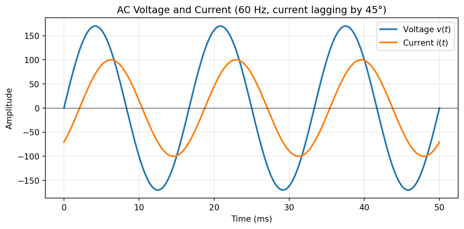
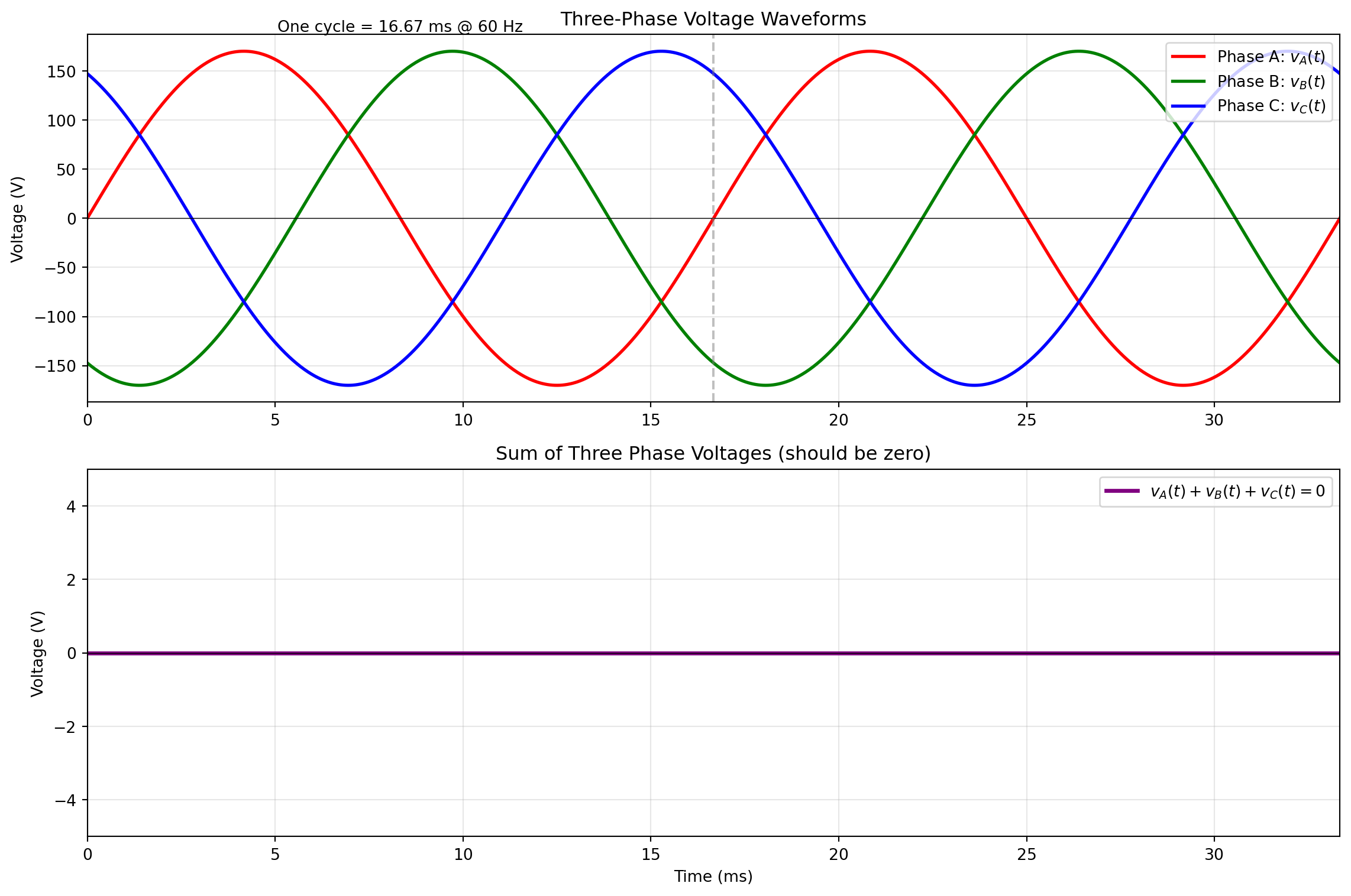
The first task is to identify cycle boundaries. We do this by detecting upward zero-crossings of the voltage signal — instants where \(v[n]\) transitions from negative to positive. Voltage zero-crossings are preferred over current zero-crossings because the voltage waveform is typically much closer to a pure sinusoid (it is set by the grid, not distorted by individual loads), making the crossings sharper and less susceptible to noise.

The time between two consecutive upward zero-crossings gives the period \(T\), and hence the line frequency \(f = 1/T\). In the US grid, we expect \(T \approx 16.67\) ms (\(f \approx 60\) Hz), though the actual value fluctuates slightly. These zero-crossings also define the boundaries of each cycle for the calculations that follow.

Step 2: Compute instantaneous and average (active) power

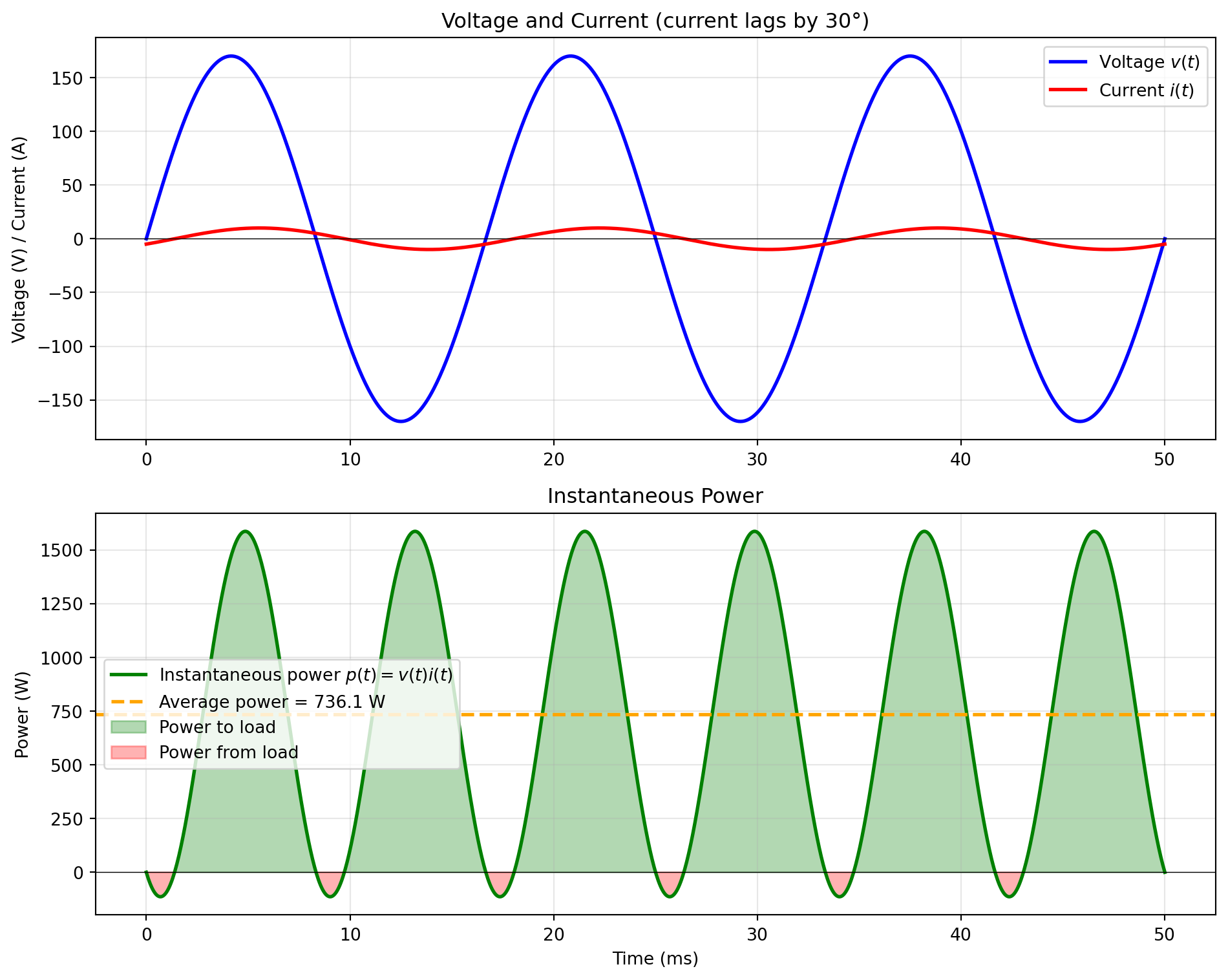
Instantaneous power at each sample is simply the product:

\[p[n] = v[n] \cdot i[n]\]

The active power (average power) over one complete cycle of \(N\) samples is:

\[P = \frac{1}{N}\sum_{n=0}^{N-1} p[n]\]

It is important to sum over complete cycles — starting and ending at the zero-crossings identified in Step 1. Averaging over a fractional cycle would allow the oscillating component to leak into the estimate, biasing the result.

Step 3: Compute RMS values and apparent power

The RMS voltage and current over the same complete cycle are:

\[V_{rms} = \sqrt{\frac{1}{N}\sum_{n=0}^{N-1} v[n]^2} \qquad I_{rms} = \sqrt{\frac{1}{N}\sum_{n=0}^{N-1} i[n]^2}\]

From these, the apparent power is:

\[S = V_{rms} \cdot I_{rms}\]

Step 4: Estimate the phase difference

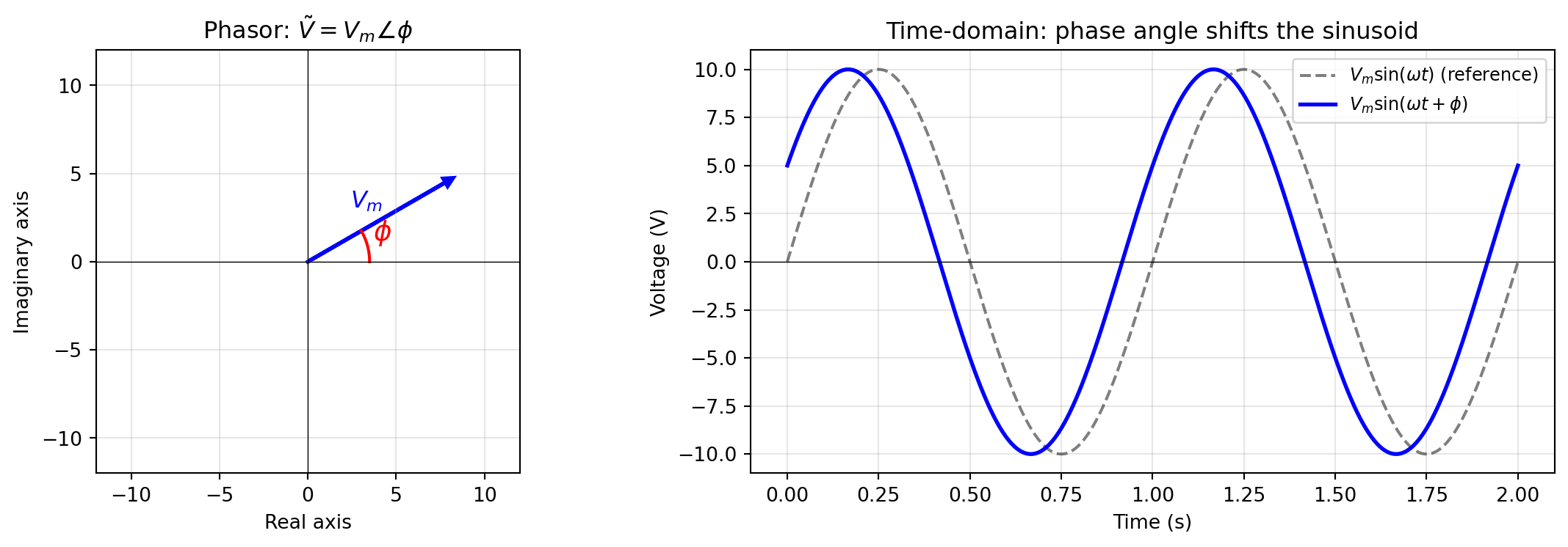
The phase angle \(\phi\) between voltage and current can be estimated from the time delay between their respective zero-crossings. If the voltage upward zero-crossing occurs at time \(t_v\) and the nearest current upward zero-crossing occurs at time \(t_i\), then:

\[\phi \approx \omega \cdot (t_v - t_i) = 2\pi f \cdot (t_v - t_i)\]

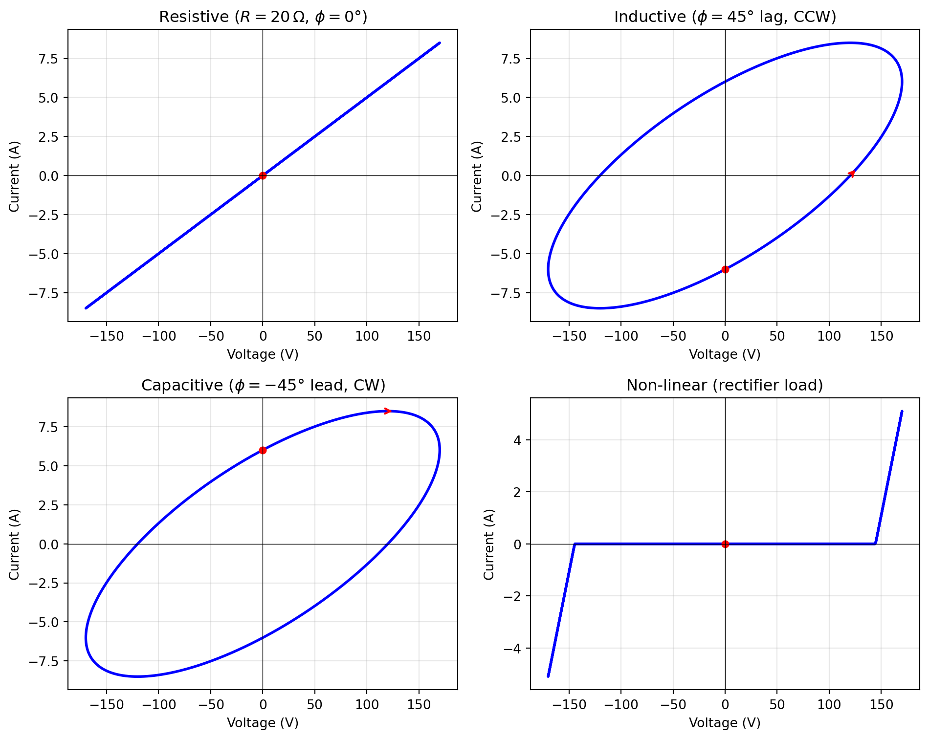
A positive \(\phi\) (current zero-crossing after voltage) indicates current lagging voltage (inductive load); a negative \(\phi\) indicates current leading (capacitive load). Note that current zero-crossings can be noisier than voltage zero-crossings, especially for loads with significant harmonic distortion, so this estimate may need filtering or averaging over several cycles.

Step 5: Close the power triangle

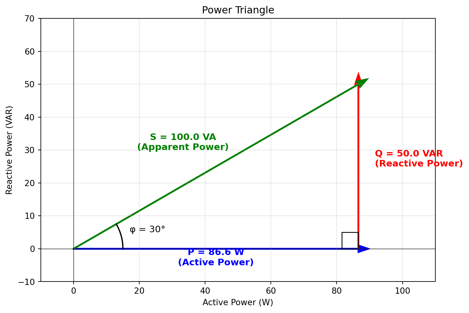
With active power \(P\) from Step 2 and apparent power \(S\) from Step 3, we can compute the remaining quantities:

\[Q = \sqrt{S^2 - P^2}\]

The sign of \(Q\) is determined by the phase difference from Step 4: positive for inductive (lagging), negative for capacitive (leading). The power factor follows directly:

\[\text{PF} = \frac{P}{S}\]

We now have the complete power triangle — \(P\), \(Q\), \(S\), and \(\text{PF}\) — derived entirely from raw voltage and current samples.

A note on redundancy and uncertainty: Strictly speaking, the power triangle is defined by three quantities (\(P\), \(Q\), \(S\)) linked by the constraint \(S^2 = P^2 + Q^2\), so only two independent estimates are needed to determine the third. In the steps above, we computed \(P\) (from instantaneous power), \(S\) (from RMS values), and \(\phi\) (from zero-crossings) — more information than the triangle requires. In principle, any pair would suffice: \(P\) and \(S\), or \(P\) and \(\phi\), or \(S\) and \(\phi\). However, each of these estimates carries its own measurement uncertainty — from quantization, sensor noise, waveform distortion, and finite sample windows. “Closing” the triangle from different pairs of quantities will generally yield slightly different results for the third. Formally, if we could quantify the uncertainty in each estimate, we could choose the pair that minimizes the propagated uncertainty in the derived quantity. In practice, \(P\) (from the average of \(v[n] \cdot i[n]\)) tends to be the most robust estimate because the sample-by-sample product and averaging operation is relatively insensitive to noise, while the phase angle \(\phi\) from zero-crossing differences tends to be the least reliable, especially for distorted current waveforms.

Practical considerations

All of the above assumes approximately steady-state conditions over the analysis window. In a real building, loads switch on and off, motors ramp up, and the grid voltage fluctuates. Keeping the analysis window short — typically a few cycles (e.g., 3–10 cycles, or roughly 50–170 ms at 60 Hz) — helps ensure that the steady-state assumption holds reasonably well within each window. Longer windows improve noise averaging but risk blurring transient events.

10.2.10.2.2 From RMS Measurements

When a metering IC or power analyzer has already computed \(V_{rms}\), \(I_{rms}\), and the phase angle \(\phi\) for us, obtaining the power triangle quantities is straightforward — we simply apply the definitions directly:

\[P = V_{rms} \, I_{rms} \cos(\phi) \qquad Q = V_{rms} \, I_{rms} \sin(\phi) \qquad S = V_{rms} \, I_{rms}\]

\[\text{PF} = \frac{P}{S} = \cos(\phi)\]

A smart meter reports \(V_{rms} = 121.3\) V, \(I_{rms} = 8.4\) A, and \(\phi = 22°\) (current lagging) for a residential circuit. Then:

  • \(S = 121.3 \times 8.4 = 1018.9\) VA
  • \(P = 1018.9 \times \cos(22°) = 944.7\) W
  • \(Q = 1018.9 \times \sin(22°) = 381.5\) VAR (inductive)
  • \(\text{PF} = 0.927\) lagging

The same steady-state caveat applies here: these RMS values are only meaningful if the underlying voltage and current were approximately constant over the measurement window. Most metering ICs update their registers every cycle or every few cycles (roughly 16–50 ms at 60 Hz), which is short enough for typical steady-state loads. However, if loads are switching rapidly — for example, a compressor cycling on — the reported RMS values may represent a blend of two different operating states. When precise transient analysis is needed, the sub-cycle approach described above gives finer temporal resolution.

10.2.11 VI Trajectory: Visualizing Load Characteristics

So far we have analyzed AC power using time-series plots — voltage and current as functions of time. But there is another way to visualize a load’s electrical behavior that is often more revealing: plotting current against voltage over one complete AC cycle. The resulting curve is called a VI trajectory (or VI signature), and its shape encodes the load’s impedance characteristics at a glance.

Use the interactive tool below to build intuition. Adjust the resistance \(R\) and reactance \(X\) of a load and observe how the VI trajectory changes shape.

Figure 10.7: Interactive VI trajectory — adjust R and X to see how the load signature changes

What to look for:

  • Straight line (when \(X = 0\)): Voltage and current are in phase — a purely resistive load. The slope of the line is \(1/R\) (steeper = lower resistance = more current).
  • Ellipse (when \(X \neq 0\)): The phase shift between voltage and current opens the trajectory into an ellipse. A wider ellipse means a larger phase angle and more reactive power.
  • Tilt direction: For inductive loads (\(X > 0\)), current lags voltage and the ellipse traverses counterclockwise. For capacitive loads (\(X < 0\)), current leads and the ellipse traverses clockwise.
  • Ellipse area: Proportional to the reactive power \(Q\) — a wider ellipse means more energy “sloshing” back and forth without doing useful work.

10.2.11.1 What is a VI Trajectory?

A VI trajectory is a parametric plot of current \(i(t)\) versus voltage \(v(t)\) over one complete AC cycle, with time as the implicit parameter. Unlike time-series plots — which show voltage and current separately as functions of time — the VI trajectory captures their relationship directly in a single curve.

For a linear load with impedance \(Z = R + jX\), the trajectory is described by the parametric equations:

\[v(\theta) = V_m \sin(\theta), \qquad i(\theta) = I_m \sin(\theta - \phi)\]

where \(\theta = \omega t\) sweeps from \(0\) to \(2\pi\) over one cycle. This parametric curve is always an ellipse (you can verify this by eliminating \(\theta\) from the two equations). The degenerate case \(\phi = 0\) collapses the ellipse into a straight line — as you can observe in the interactive tool above by setting \(X = 0\).

The power of VI trajectories lies in their compactness: a single curve encodes the load’s impedance magnitude (through the current amplitude), phase relationship (through the ellipse shape), and power characteristics (through the ellipse area). This makes them particularly useful as “fingerprints” for identifying different types of electrical loads, as we discuss next.

10.2.11.2 VI Trajectories for Different Load Types

The shape of a VI trajectory is determined by the type of load. For linear loads, the trajectory is always an ellipse (or a line), but non-linear loads produce more complex shapes. The figure below shows representative trajectories for four common load types.

Figure 10.8: VI trajectories for four load types: resistive (straight line), inductive (ellipse, CCW), capacitive (ellipse, CW), and non-linear (complex shape)

Resistive load (top left): The trajectory is a straight line through the origin. Voltage and current are perfectly in phase — when voltage is positive, current is positive, and vice versa. The slope of the line equals \(1/R\). Examples: incandescent light bulbs, resistive space heaters, electric water heater elements.

Inductive load (top right): The trajectory opens into an ellipse. Current lags voltage, so the ellipse is traversed counterclockwise (indicated by the arrow). The wider the ellipse, the larger the phase angle and the more reactive power the load draws. Examples: induction motors, fans, transformers, fluorescent lighting ballasts.

Capacitive load (bottom left): Also an ellipse, but now current leads voltage and the trajectory is traversed clockwise. Pure capacitive loads are less common in buildings, but capacitor banks used for power factor correction produce this signature. Some electronic power supplies also exhibit a leading power factor.

Non-linear load (bottom right): The trajectory departs from the smooth elliptical shape entirely. The example shown simulates a rectifier with a capacitor filter — the type of front-end found in most computers, phone chargers, and LED drivers. Current flows only in brief pulses near the voltage peaks (when the supply voltage exceeds the capacitor voltage), producing a distinctive “pinched” shape with sharp features. For these loads, the simple \(Z = R + jX\) model no longer applies, and a full harmonic analysis is needed to characterize their behavior.

10.2.11.3 Using VI Trajectories for Load Identification

Since different load types produce distinct VI trajectory shapes, these trajectories can serve as electrical fingerprints for identifying what appliance is running. This insight is the foundation of Non-Intrusive Load Monitoring (NILM) — a technique where a single sensor installed at the electrical panel monitors the aggregate voltage and current, and algorithms decompose the combined signal to identify and track individual loads without requiring a sensor on each appliance.

In practice, a NILM system works by building a library of reference VI trajectories for known appliance types (e.g., a refrigerator compressor, a microwave, a laptop charger). When the system detects a change in the aggregate signal — such as a new load turning on — it extracts the VI trajectory of the change and compares it against the library using pattern matching or machine learning classifiers. Variations of this approach have been applied to residential energy disaggregation, fault detection in commercial buildings, and industrial equipment monitoring. NILM remains an active research area, with ongoing work on improving accuracy, handling multiple simultaneous events, and scaling to diverse building types.

That said, VI-based load identification has practical limitations. When multiple loads operate simultaneously, the measured trajectory is a superposition of individual trajectories, making decomposition challenging. Loads of the same type (e.g., two different induction motors) may produce similar trajectories that are hard to distinguish. And loads that operate in variable or transient modes — such as a washing machine cycling through different stages — produce time-varying trajectories that don’t fit neatly into a single-cycle fingerprint. Despite these challenges, VI trajectories remain one of the most intuitive single-cycle representations of electrical load behavior.

10.3 Additional Resources

10.3.1 References