viewof frequency = Inputs.range([0.25, 10], { step: 0.25, value: 1, label: "Frequency (cycles per day)" });
viewof samplingRate = Inputs.range([0.125,10], { step: 0.125, value: 1, label: "Sampling Rate (measurements per hour)" });
viewof showSineWave = Inputs.toggle({ label: "Show Continuous Sine Wave", value: true }); // New toggle button

t = Array.from({ length: 2400 }, (_, i) => i * 0.01); // Time array for continuous plot from 0 to 24 hours

// Continuous sine wave
continuous = t.map(t => ({ t, x: 1 + Math.sin(2 * Math.PI * (frequency / 24) * t) }));

// Sampled sine wave
sampled = Array.from({ length: Math.floor(24 * samplingRate) + 1 }, (_, i) => {
  const time = i / samplingRate;
  return { t: time, x: 1 + Math.sin(2 * Math.PI * (frequency / 24) * time) };
});

// Plotting
Plot.plot({
  x: { domain: [0, 24], label: "Time (hours)" },
  y: { label: "x(t)" },
  marks: [
    showSineWave ? Plot.line(continuous, { x: "t", y: "x", stroke: "blue" }) : null, // Conditional rendering of sine wave
    Plot.dot(sampled, { x: "t", y: "x", stroke: "red", fill: "red" }) // Sampled points
  ]
})5 Review of Data Acquisition and Instrumentation
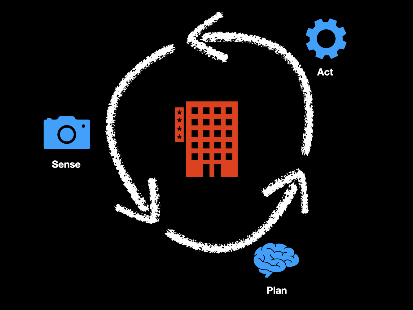
Since for a building to be autonomous, it needs to be able to sense, plan, and act; then we need to review the principles of sensing in more detail. That is what we will do today.
5.1 Defining Autonomous Sustainable Buildings
Understanding the three terms in the title of this course (i.e., Autonomous, Sustainable and Buildings) is important before moving any further. In particular, the first two terms need to be defined ahead of time since buildings are a familiar object and we will spend a great deal discussing their inner workings in upcoming chapters. So what do we mean by a building that is autonomous and sustainable?
We can argue at length about the specific definition for these two terms so I want to start by pointing out that the specific definition is not that important (at least not right now). Instead, I find it more important for us to agree on the fact that sustainability is a goal, and that autonomous technologies are those that can achieve goals set by humans with minimal assistance from them. From this perspective, what we mean by the words in the title of the course is that its scope is defined by the technologies needed to allow buildings to achieve sustainable goals with minimal human intervention. Sustainability, of course, is a wide concept but Wikipedia’s definition seems appropriate for us: “Sustainability is a societal goal that relates to the ability of people to safely co-exist on Earth over a long time”. It is also worth pointing out that autonomy, in our view, is distinctly different from automation. While the latter refers to the ability of a system/process to execute some specific sequence of steps on its own, the latter refers to the ability of the system/process to not only enact those steps but also determine what they should be in the context of a given goal. This is, at least, our definition of these terms.
Autonomous systems follow a three-step cycle: sense, plan and act. Sensing refers to the ability of the system to perceive its environment and itself and develop some situational awareness. Planning (which in many contexts also includes learning), refers to the ability of the system to develop models of the world and itself based on the observations collected through sensing, as well as using these models to reason. Lastly, the actuation step allows the system to intervene and cause an effect in the environment, as decided upon by the planning step.
5.2 Sensors
Given that our goal in the course is to create autonomous technologies to reach sustainability goals in buildings, we will need to focus our attention on this trifecta: sense, plan, act; and understand how it applies in the context of buildings. This chapter is intended to serve as a refresher for the main ideas behind modern sensing systems. For a more thorough treatment of this topic, we refer the reader to Fraden (2010), specifically Chapters 1 and 2. What follows is an abridged account of the main ideas needed to understand modern sensors and the process of turning analog signals into digital ones that can be processed by computers.
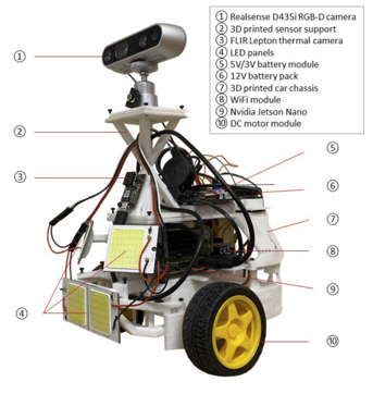
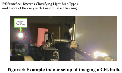
To start, let’s take a look at some example sensing systems (which may do much more than just sensing) that have been developed in the last few years to tackle some building energy management problems:
Modern sensors and actuators are a relatively inexpensive commodity that has benefited tremendously from the technological advances of the past century to become cheap, miniaturized, reliable and massively produced. Most people living in the world today interact with sensors in one way or another and many carry multiple sensors in their pockets (e.g., on their mobile devices) all day. For our purposes, in this course, sensors are devices that can convert a physical stimulus into an electrical signal; actuators are devices that convert an electrical signal into a physical stimulus (the inverse of a sensor); and we can call either of these a transducer (i.e., a transducer is a term encompassing both sensors and actuators) and this term extends to include non-electrical devices too.
Given their wide availability and low-cost, there are a number of resources you can use to find sensors for your project in this course. Since we are going to be using Raspberry Pi computing platforms, here is a good starting point for finding sensing hardware:
- Raspberry Pi Hardware by Adafruit
- Best Raspberry Pi HATs in 2023 by Tom’s Hardware
- Raspberry Pi HATs, pHATS & GPIO by Pihut
- Rasbperry Pi Pico Hardware by Pimoroni
You should start thinking about what kinds of sensors you want to use for your project (if you know what its goal is), or get inspired by these sensors to define a goal for your project.
5.3 Digitizing Analog Signals
If sensors convert a physical stimulus into an electrical signal, how do we reason about that electrical signal to enable the planning and actuation phase of the autonomous solution we are designing? The answer, of course, is through the use of computers (broadly speaking, not just the electronic digital ones based on the von Neumann architecture we see everywhere today). That said, because our most successful approach at creating computers is based on digital electronics and the electrical signals that the sensors are producing will likely be analog, we need to involve (among other things) an analog-to-digital converter (ADC, or A/D converter) in the process. The topic of ADCs is wide and deep, and we are assuming in this course that you will have had some prior exposure to it. However, if you have not been exposed to it the minimum requirements for you to continue understanding the rest of the material are a basic understanding of the digitization process, in particular: sampling and quantization.
Since digital electronics process discrete information (bits), we need to discretize our incoming analog signal in both both time and magnitude. The process of discretizing time is called sampling, while the process of turning a continuous amplitude into a finite discrete set is called quantization.
5.3.1 Sampling
Let’s start with the discretization of time. The interactive plot below shows a simple sine wave \(x(t) = 1 + sin(2\pi\frac{f}{24}t)\) where \(f\) is the frequency of the sine wave and \(t\) is time measured in hours (the period of this signal is 24 hours, as you may have noticed). Let’s imagine that this sinusoid is the physical phenomenon we are interested in measuring. This could be any property of the physical system we are twinning which, through a specific sensor, we are able to convert into an electrical signal. A simple example, in keeping with is that \(x(t)\) represents the response of a photoresistive sensor sitting on the window as the sun goes up and down each day. If we take snapshots, or measurements of this signal at equally-spaced time intervals, the amount of time in between these measurements has a very important role to play in our ability to accurately represent the physical phenomenon we are measuring.
You can prove this to yourself by interacting with the simple simulation below.
Simply playing around with this can be very useful towards building intuition. But it helps to follow some directions, so you may want to wait until the activity at the end of this module for some specific guidance and suggestions for what to try.
5.3.2 Quantization
As we said initially, sampling is just one of the discretizations we need to do. But in addition to discretizing time, we also need to discretize the continuous amplitude of the analog signal through a process called quantization. Just as with sampling, quantization can introduce additional errors to our measurements. So it is worth paying close attention to how this process works in order to understand the possible errors. For instance, imagine that we continue trying to measure the intensity of light outside as driven by the day/night cycle on Earth. In the previous example we imagined that no matter when we measured the light intensity, our measurement apparatus would be able to provide us with the exact number representing the magnitude of light intensity at that moment. But what if we can only express that magnitude crudely, say by considering if it is “dark”, “dimly lit”, “bright” and “very bright” but nothing else? Well, it is obvious that this would be far from ideal to understand precisely how light intensity varies throughout the day.
Again, to build intuition regarding this concept, it helps to play around with the effects. The simulation below allows you to do just that:
Activity: Exploring the Effects of Sampling and Quantization on Signal Accuracy
Use the interactive plot to experiment with signal sampling and quantization. Your goal is to understand how poorly chosen parameters can affect the measurement of a signal.
Instructions:
Start by hiding the continuous signal (toggle “Show Continuous Sine Wave” off).
Set the sliders to the following values for each case and observe the plotted points:
- Case 1: Quantization levels = 8, Frequency = 6.75, Sampling rate = 1.
- Case 2: Quantization levels = 2, Frequency = 11, Sampling rate = 1.
- Case 3: Quantization levels = 16, Frequency = 10, Sampling rate = 0.375.
After exploring each case, answer the following:
- How do the sampled points differ from the original signal?
- How does reducing the quantization level or sampling rate affect the usefulness of the measurements?
- What are the key differences in signal behavior across the three cases?
5.4 What have you learned?
After the lecture, here are some questions that you may want to try to answer yourself to see if you really understood things.
Technical Questions
- According to the Nyquist-Shannon sampling theorem, if we want to sample a 100Hz signal, what sampling frequency should we use?
- What is the resolution of a 16-bit ADC with a 10V full-rage voltage input?
- If I sample a pure 100Hz signal at 60Hz, at what frequency does the resulting discrete signal repeat itself?
- What are HATs in the context of Raspberry Pis and other embedded systems?
- In the context of cars, which of the following is an example of an autonomous technology: cruise control, lane-keep assist, automatic parking.